Binary image segmentation using the level set method

Image segmentation is the task of splitting a digital image into one or more areas of interest. This is a fundamental problem in the field of computer vision, which is solved in many different ways, each of which has its own advantages and disadvantages.

In this article I will briefly review the concept of a method of fixing a level and implicitly defined dynamic surfaces (level set method). I will also consider the role of this method in binary segmentation with the introduction and definition of mathematical constructions, such as SDT (Signed Distance Transforms), a marked distance map.

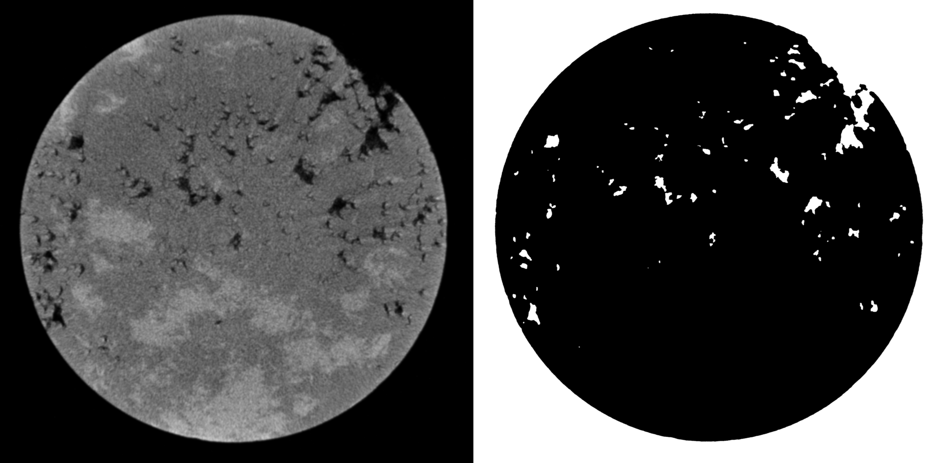
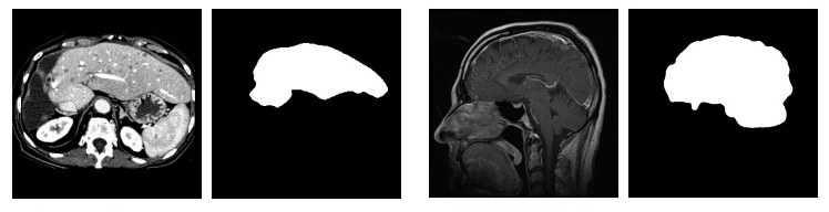On the left - the original image, on the right - segmented

Why all this?

In various industries, there is often a need for segmented images. For example, in medicine, where there is an interest in obtaining digital 3D models of organs for further analysis. Segmentation is also used in face recognition , machine vision , etc.
')
Image segmentation is a particularly difficult task for several reasons. First, at present there are no universal segmentation algorithms, therefore it is necessary to create special algorithms, the parameters of which are selected by the user, based on specific conditions. Secondly, image distortions such as noise, inhomogeneity, etc., are very difficult to take into account in segmentation algorithms without user intervention.

The second problem is usually fought using different types of filters. This technology is perfectly described here .

I was faced with the task of image segmentation in the oil and gas industry. Initially, we had flat core images (as in the figure above). Having obtained a segmented image, we can interpolate the borders. Having performed this operation for all images, we can get a mathematical model of our rock sample, with which we can work and on which, for example, we can set the flow of fluids (if we consider our model as a model of continuum mechanics).

Level fixation method

This method was introduced by American mathematicians Stanley Osher and James Setian in the 1980s. It has become popular in many disciplines, such as computer graphics, image processing, computational geometry, optimization, computational fluid dynamics, and computational biophysics.

The level fixation method implicitly transforms the contour (in two dimensions) or surface (in three dimensions) using a higher dimension function, called the level fix function $$$φ (x, t)$ . Converted contour or surface can be obtained as a curve $$$\ Gamma (x, t) = \ {φ (x, t) = 0 \}$ .
The advantage of using this method is that topological changes, such as merging and separating a contour or surface, are implicitly solved, as shown in the figure below.

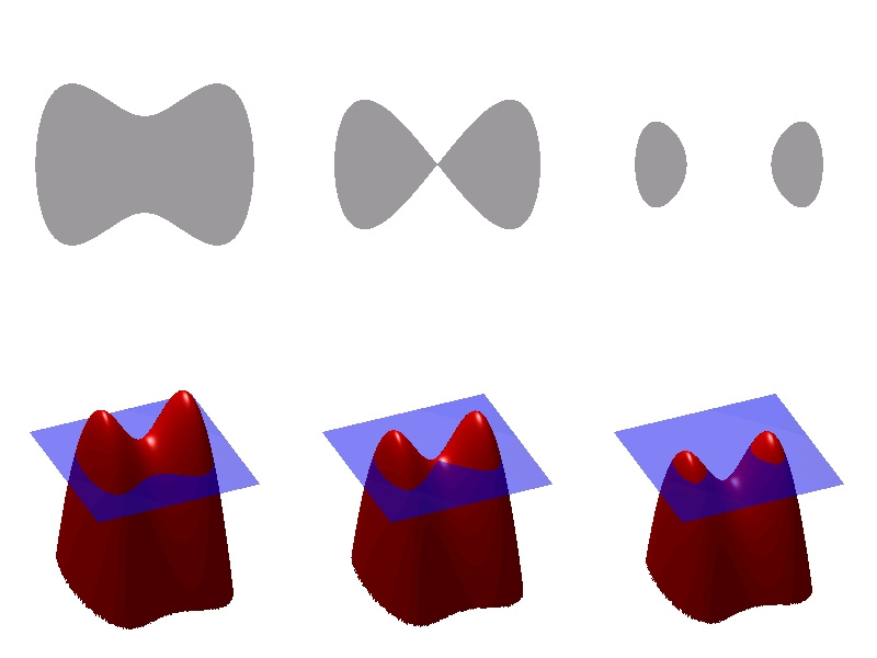
You can see the relationship between the level fixation function (bottom) and the contour (top). It is seen that the change in the surface breaks the contour.

Level modification equation

The definition of a contour or surface is determined by the equation of level modification. We obtain a numerical solution of this partial differential equation by updating $$$φ$ for each temporary layer. The general view of the level modification equation is:

$$$$ display $$ \ frac {∂φ} {∂t} = -F | ∇φ | \ qquad (1) $$ display $$

Where:
$$$| · |$ - Euclidean norm,
$$$φ$ - function of fixing the level
$$$t$ - time
$$$F$ - speed ratio.

This partial differential equation is very similar to hyperbolic. But due to the fact that on the right side of the equation, in addition to the derivative in space, there is also a derivative in time, strictly speaking, it is not.

With a specific task type of vector $$$F$ up to parameters, we can direct the level line to different areas or shapes.

For applications in segmentation we will ask $$$F$ So:

$$$$ display $$ F = αD (I) + (1-α) ∇ \ cdot \ frac {∇φ} {| ∇φ |} \ qquad (2) $$ display $$

Where:

$$$D (i)$ - data function, which leads decisions to the desired segmentation,
$$$I$ - pixel intensity value,
$$$ inline $ ∇ \ cdot \ frac {∇φ} {| ∇φ |} $ inline $ - the middle term of the curvature of the function $$$φ$ that will keep this function smooth,
$$$\ alpha$ - weight parameter.

Data function $$$D (i)$ acts as the main “force” that controls segmentation. By doing $$$D$ positive in the desired areas or negative in the undesired, the model will tend to the desired segmentation. Here is a simple data function:

$$

$$D (I) = ε- | I-T | \ qquad (3)$$

Her work is shown below in the figure:


That is, if the pixel value falls within the interval $$$(T - ε, T + ε)$ , then the range of the model will expand, otherwise - to narrow.

Therefore, the three user parameters that must be specified for segmentation are $$$T,$ ε and $$$\ alpha$ .
For example, if we need to select objects with a low level of brightness (black areas) in the image, then $$$T$ is chosen equal to zero.


On the left, select the black areas, on the right, the desired area has a higher brightness, so select $$$T = $ 4$

Initial mask is also required. $$$m$ . From what we choose it, will depend on the initial approximation $$$φ$ . To do this, we introduce the concept of a marked distance map.

Signed Distance Transforms

The distance map is a matrix that has the same dimension as our image. It is constructed in the following way: for each pixel of our image, a value equal to the minimum distance from this pixel to the nearest pixel on the border of the object (s) is calculated. Mathematical definition of the distance function $$$d: R ^ 3 \ to R$ for set S:

$$

$$d (r, s) = min | r-s | \ qquad for all \ qquad r∈R ^ 3$$

Marked distance map is a matrix that has a positive sign in front of the pixel values ​​that are outside the object, and negative for those inside it. This agreement is a sign that will be implemented during the implementation, but the opposite convention of the sign could also be used. It should be noted that the cell values ​​depend on the selected metric: some common distance metrics are Euclidean distance, Chebyshev distance (Chebyshev distance, chessboard distance) and city ​​blocks distance (Taxicab geometry, city block distance, Manhattan distance) .


On the left we choose the initial mask. This is an object of any form, located inside the object of interest to us. Most often it is a rectangle, because it is pretty easy to set. After a certain number of iterations, the function on the right (the level modification function) changes in such a way that its intersection with the zero plane gives the curve of interest

Sampling

Equation (1), the level equation, must be discretized for sequential or parallel computation. This is done using a difference circuit with upwind differences.

The method of the first order of accuracy for the time discretization of equation (1) is given by the direct Euler method:

$$$$ display $$ \ frac {(φ ^ {t + ∆t} -φ ^ t)} {∆t} + F ^ t \ cdot∇φ ^ t = 0 \ qquad (4) $$ display $$

Where:

$$$φ ^ t$ - current values $$$φ$ at the moment of time $$$t$
$$$F ^ t$ - velocity vector at time $$$t$
$$$∇φ ^ t$ - gradient values $$$φ$ at the moment of time $$$t$

In calculating the gradient, great care must be taken with respect to spatial derivatives. $$$φ$ . This is best seen if we consider the extended form of equation (4):

$$$$ display $$ \ frac {(φ ^ {t + ∆t} -φ ^ t)} {∆t} + u ^ t φ_x ^ t + v ^ t φ_y ^ t + w ^ t φ_z ^ t = 0 \ qquad (5) $$ display $$

Where $$$u, v, w$ - Components $$$x, y, z$ of $$$F$ . For simplicity, consider the one-dimensional form of equation (5) at a particular grid point. $$$x_i$ :

$$$$ display $$ \ frac {(φ ^ {t + ∆t} -φ ^ t)} {∆t} + u_i ^ t \ cdot (φ_x) _i ^ t = 0 \ qquad (6) $$ display $$

Where $$$(φ_x) _i ^ t$ - derivative $$$φ$ space at point $$$x_i$ . In order to understand what difference scheme to use, direct or inverse, we will be based on the sign $$$u_i$ at the point $$$x_i$ . If a $$$u_i> 0$ values $$$φ$ move from left to right, and therefore you should use inverse difference schemes ( $$$D_x ^ -$ in equations 7). On the contrary, if $$$u_i <0$ then for approximation $$$φ_x$ should use direct difference schemes ( $$$D_x ^ +$ in equations 7). It is this selection process of the approximation for the derivative $$$φ$ in space based on the sign $$$u_i$ , is known as flow calculation .

In the two-dimensional case to calculate $$$φ$ we need the derivatives listed below. It is worth mentioning that we make the assumption that the image is isotropic.

$$$$ display $$ \ begin {matrix} D_x = \ frac {φ_ {i + 1, j} -φ_ {i-1, j}} 2 \ qquad D_x ^ + = \ frac {φ_ {i + 1, j } -φ_ {i, j}} 2 \ qquad D_x ^ - = \ frac {φ_ {i, j} -φ_ {i-1, j}} 2 \\ D_y = \ frac {φ_ {i, j + 1 } -φ_ {i, j-1}} 2 \ qquad D_y ^ + = \ frac {φ_ {i, j + 1} -φ_ {i, j}} 2 \ qquad D_y ^ - = \ frac {φ_ {i , j} -φ_ {i, j-1}} 2 \ end {matrix} \ qquad (7) $$ display $$

$$$∇φ$ approximated using the upwind scheme:

$$

$$∇φ_ {max} = \ begin {bmatrix} \ sqrt {max (D_x ^ +, 0) ^ 2 + max (-D_x ^ -, 0) ^ 2} \\ \ sqrt {max (D_y ^ +, 0 ) ^ 2 + max (-D_y ^ -, 0) ^ 2} \ end {bmatrix} \ qquad (8)$$

$$

$$∇φ_ {min} = \ begin {bmatrix} \ sqrt {min (D_x ^ +, 0) ^ 2 + min (-D_x ^ -, 0) ^ 2} \\ \ sqrt {min (D_y ^ +, 0 ) ^ 2 + min (-D_y ^ -, 0) ^ 2} \ end {bmatrix} \ qquad (9)$$

Finally, depending on whether $$$F_ {i, j, k}> 0$ or $$$F_ {i, j, k} <0$ , $$$∇φ$ It seems like:

$$$$ display $$ ∇φ = \ begin {cases} ‖∇φ_ {max} ‖_2 & \ quad \ text {if} F_ {i, j, k}> 0 \\ φ_ {min} _2 & \ quad \ text {if} F_ {i, j, k} <0 \\ \ end {cases} \ qquad (10) $$ display $$

$$$$ display $$ φ (t + Δt) = φ (t) + ΔtF | ∇φ | \ qquad (11) $$ display $$

The velocity factor F, as previously discussed, is based on pixel intensity values ​​and curvature values.

Curvature

We will calculate it on the basis of the values ​​of the current level, established using the following derivatives. In two dimensions only $$$D_x ^ {+ y}, D_x ^ {- y}, D_y ^ {+ x}, D_y ^ {- x}$ , along with previously defined derivatives:

$$$$ display $$ \ begin {matrix} D_x ^ {+ y} = \ frac {(φ_ {i + 1, j + 1} -φ_ {i-1, j + 1})} 2 \ qquad D_x ^ { -y} = \ frac {(φ_ {i + 1, j-1} -φ_ {i-1, j-1})} 2 \\ D_y ^ {+ x} = \ frac {(φ_ {i + 1 , j + 1} -φ_ {i + 1, j-1})} 2 \ qquad D_y ^ {- x} = \ frac {(φ_ {i-1, j + 1} -φ_ {i-1, j -1})} 2 \ end {matrix} \ qquad (12) $$ display $$

Using the normal difference, the curvature is calculated using the above derivatives with two normals. $$$n ^ +$ and $$$n ^ -$ .

$$

$$n ^ + = \ begin {bmatrix} \ frac {D_x ^ +} {\ sqrt {(D_x ^ +) ^ 2 + (\ frac {D_y ^ {+ x} + D_y} {2}) ^ 2}} \\ \ frac {D_y ^ +} {\ sqrt {(D_y ^ +) ^ 2 + (\ frac {D_x ^ {+ y} + D_x} {2}) ^ 2}} \\ \ end {bmatrix} \ qquad (13)$$

$$

$$n ^ - = \ begin {bmatrix} \ frac {D_x ^ -} {\ sqrt {(D_x ^ -) ^ 2 + (\ frac {D_y ^ {- x} + D_y} {2}) ^ 2}} \\ \ frac {D_y ^ -} {\ sqrt {(D_y ^ -) ^ 2 + (\ frac {D_x ^ {- y} + D_x} {2}) ^ 2} \ \ end {bmatrix} \ qquad (14)$$

Two normals are used to calculate the divergence, with which we calculate the mean curvature, as shown below:

$$$$ display $$ H = \ frac {1} {2} ∇ \ cdot \ frac {∇φ} {| ∇φ |} = \ frac {1} {2} ((n_x ^ + - n_x ^ -) + (n_y ^ + - n_y ^ -)) \ qquad (15) $$ display $$

Resilience

Stability arises from the Courant-Friedrichs-Levy (CFL) condition, which states that the speed of information in a computational scheme must be such that during $$$∆t$ you do not go beyond a single cell, that is $$$\ frac {∆x} {∆t}> | u |$ . We have:

$$

$$∆t <\ frac {∆x} {max {| u |}} \ qquad (16)$$

Sequential implementation

We implement this binary segmentation algorithm in the Matlab system. Let's do this, first of all, for clarity, since Matlab does an excellent job with working with tables. Also there are very simple functions that allow you to read images and display the work of the algorithm on the screen. Thanks to this, the code will be compressed and understandable. Naturally, implementation, for example on C will be much more profitable in terms of speed. But in this article we do not pursue speed, but try to understand the method.

The pseudocode of the algorithm can be seen below:

• Input: Original image I; initial mask m; threshold t; error ε; number of iterations N; a number indicating how many iterations we recalculate the distance map, ITS.
• Output: The result of the segmentation is the seg image.
  Initialize the φ_0 with the Signed Euclidean Distance Transform (SEDT) and the m mask.
  Calculate D (I) = ε- | IT |.
• Cycle i from 1 to N
  
  • Calculate first order derivatives
  • Calculate second order derivatives
  • Calculate normal values $$$n ^ +$ and $$$n ^ -$
  • Calculate the value of the gradient $$$∇φ$
  • Calculate the value of the function$$ $ inline $ F = αD (I) + (1-α) ∇ \ cdot \ frac {∇φ} {| ∇φ |} $ inline $
  • Update level feature$$ $ inline $ φ (t + Δt) = φ (t) + Δt \ cdot F \ cdot | ∇φ | $ inline $
  • If i % ITS == 0 then
    Reinitialize $$$φ$ using sedt
    End if
  
  End of cycle

Let's start with the fact that we choose the format of images with which we will work. The PGM format was very convenient. This is an open format for storing bitmap bitmap images without compression in grayscale. It has a simple ASCII header, and the image itself is a sequence of single-byte (for shades of gray from 0 to 255) unsigned integers. More information about the format you can read directly in the standard itself, the link is given in the sources section.

We divide our code into two parts: the “launcher” and the “core” in order to separate the initialization and update code of the level set. The first file handles the download and reduces the image resolution using the imread and imresize functions. User sets parameters for threshold values. $$$T$ range $$$ε$ and curvature weighting $$$\ alpha$ , launches the launcher and then proceeds to draw a closed polygon that will form the initial mask (providing some basic interactivity).

So, we read the image and immediately create a zero matrix. $$$m$ which will be our mask:

 I = imread('test_output.pgm'); I = imresize(I, 1); init_mask = zeros(size(I,1),size(I,2)); 

To create a mask, it is convenient to choose the coordinates of the center and deviations from it. Get a rectangle filled with units. We will transfer it to the core.

 x = 400; y = 800; %   dx = 10; dy = 10; init_mask(y - dy : y + dy, x - dx : x + dx) = 1; %  seg = simpleseg(I, init_mask, max_its, E, T); %   

Now consider the function simpleseg , which is the core of the code. First you need to get the SDF from the init_mask mask:

 phi = mask2phi(init_mask); % SDF function phi = mask2phi(init_a) %  SDF phi=bwdist(init_a)-bwdist(1-init_a); 

Let's write a function that will calculate the curvature:

 %  function curvature = get_curvature(phi) dx = (shiftR(phi)-shiftL(phi))/2; dy = (shiftU(phi)-shiftD(phi))/2; dxplus = shiftR(phi)-phi; dyplus = shiftU(phi)-phi; dxminus = phi-shiftL(phi); dyminus = phi-shiftD(phi); dxplusy = (shiftU(shiftR(phi))-shiftU(shiftL(phi)))/2; dxminusy = (shiftD(shiftR(phi))-shiftD(shiftL(phi)))/2; dyplusx = (shiftR(shiftU(phi))-shiftR(shiftD(phi)))/2; dyminusx = (shiftL(shiftU(phi))-shiftL(shiftD(phi)))/2; nplusx = dxplus./sqrt(eps+(dxplus.^2 )+((dyplusx+dy )/2).^2); nplusy = dyplus./sqrt(eps+(dyplus.^2 )+((dxplusy+dx )/2).^2); nminusx= dxminus./sqrt(eps+(dxminus.^2)+((dyminusx+dy)/2).^2); nminusy= dyminus./sqrt(eps+(dyminus.^2)+((dxminusy+dx)/2).^2); curvature = ((nplusx-nminusx)+(nplusy-nminusy))/2; 

Derivatives are calculated by subtracting the shifted matrices of the function. $$$φ$ . Note that derivatives are not calculated elementwise, as this would be less efficient.

 %--       function shift = shiftD(M) shift = shiftR(M')'; function shift = shiftL(M) shift = [ M(:,2:size(M,2)) M(:,size(M,2))]; function shift = shiftR(M) shift = [M(:,1) M(:,1:size(M,2)-1)]; function shift = shiftU(M) shift = shiftL(M')'; 

Now consider the rate factor $$$F$

  alpha=0.5; D = E - abs(I - T); K = get_curvature(phi); F = alpha*single(D) + (1-alpha)*K; 

Then go to the upgrade levels. To do this, we first calculate the gradient to maintain stability:

 dxplus = shiftR(phi)-phi; dyplus = shiftU(phi)-phi; dxminus = phi-shiftL(phi); dyminus = phi-shiftD(phi); gradphimax_x = sqrt(max(dxplus,0).^2+max(-dxminus,0).^2); gradphimin_x = sqrt(min(dxplus,0).^2+min(-dxminus,0).^2); gradphimax_y = sqrt(max(dyplus,0).^2+max(-dyminus,0).^2); gradphimin_y = sqrt(min(dyplus,0).^2+min(-dyminus,0).^2); gradphimax = sqrt((gradphimax_x.^2)+(gradphimax_y.^2)); gradphimin = sqrt((gradphimin_x.^2)+(gradphimin_y.^2)); gradphi = (F>0).*(gradphimax) + (F<0).*(gradphimin); dt = .5/max(max(max(abs(F.*gradphi)))); 

And change the function set of levels $$$φ$ :

 phi = phi + dt.*(F).*gradphi; 

We will display the intermediate result on the screen every 20 iterations:

  if(mod(its,20) == 0) showcontour(I,phi,its); subplot(2,2,4); surf(phi); shading flat; end 

Using the showcontour function:

 function showcontour(I, phi, i) subplot(2, 2, 3); title('Evolution') ; imshow (I); hold on; contour(phi, [0 0],'g','LineWidth', 2); hold off ; title([num2str(i) 'Iterations'] ); drawnow; 

results

I carried out algorithm tests on two types of images: medical and images of rocks (since I solved this problem on a diploma).

For medical images, it works like this:



We see that the algorithm copes very well with this task.

It is worth saying that this algorithm can be implemented for the three-dimensional case. In this article I will not describe the features, but I will show how it works:


In this case, the initial mask is a cube (in general, of course, it is any three-dimensional body)

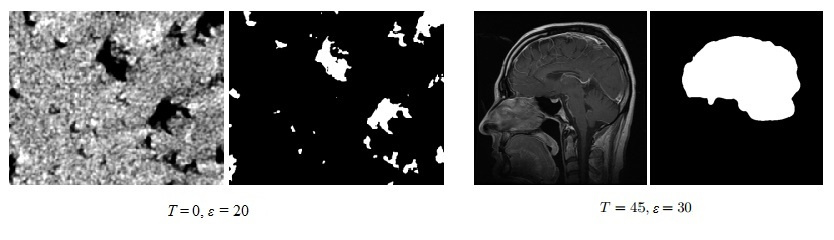
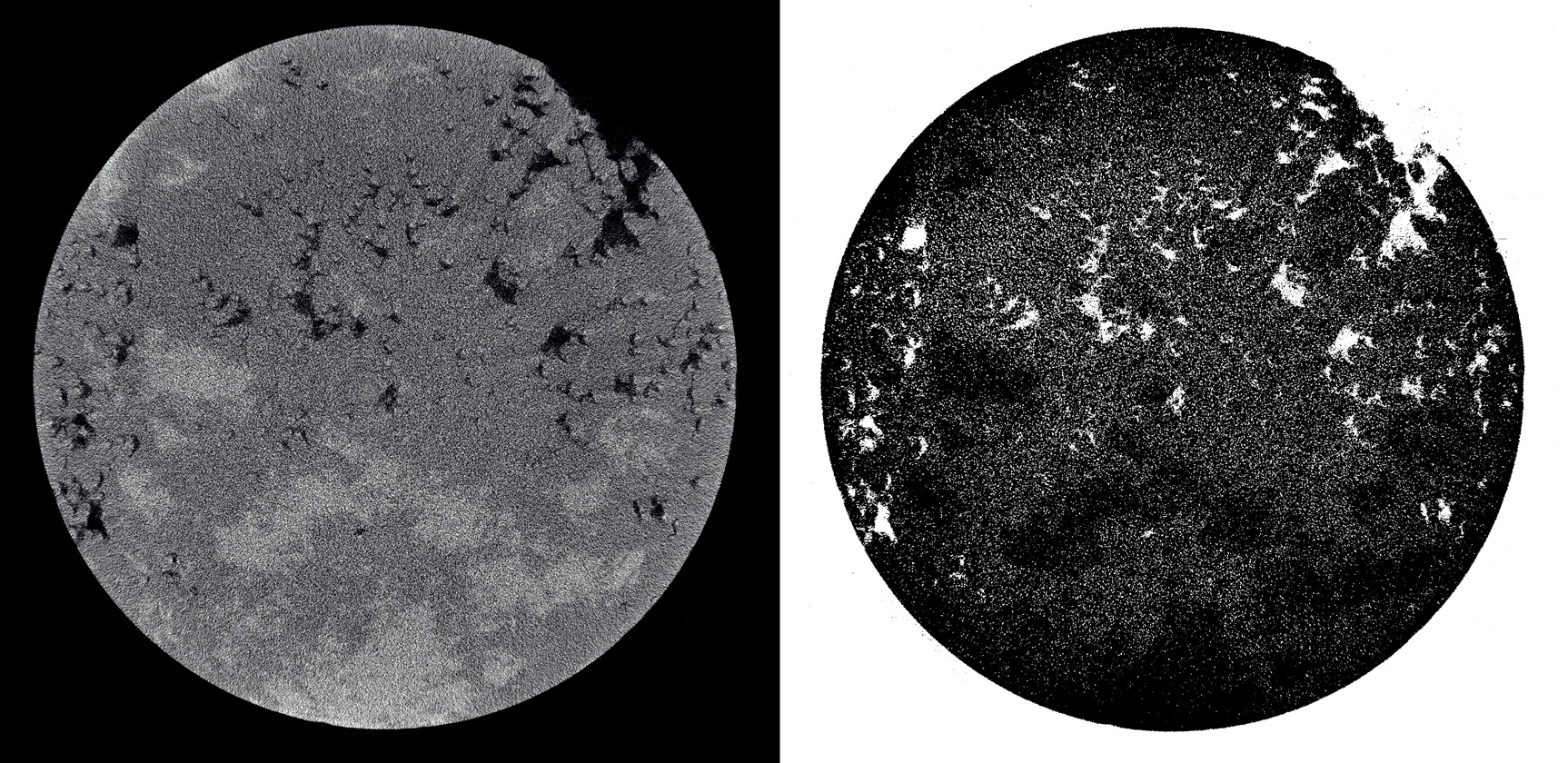
In the segmentation of images of rocks in the first place you encounter the problem of noise. This is due to many reasons: starting from the inaccuracy of tomographs, ending with errors in the inverse Radon transform (this is how such images are obtained). That is why you first need to filter the image. The Peron and Malik anisotropic diffusion filter copes with this very well. The link to the article about this filter was already at the beginning of the article. Leave it at the end of the post.

This is what happens if you segment a noisy image:



But what with the filtered image:

Conclusions and further work

The level fixation method is an excellent method for performing binary segmentation. Its main disadvantage is a large computational complexity. The time it took for Matlab to process an image of 512x512 on my machine (5000 iterations were performed) is 2737.84 seconds (45 minutes). This, of course, is incredibly much.

But do not close the article after reading this fact. The most important reason for me choosing this algorithm was that it is very well parallel. I did this with the help of CUDA, you can use something else and write about it, for example, in the comments. If someone is interested, in the future I will write the following article on the parallelization of this algorithm.

PS Here are links to source codes: the start file and the function that is directly responsible for the segmentation .

Sources

1. Wikipedia article on method
2. Filter article