Things I needed to know before creating a queue system

In the project I'm working on, a distributed data processing system is used: first, several dozen machines simultaneously produce some messages, then these messages are sent to the queue, three threads retrieve messages from the queue, and after final processing they upload data to the Redis database. At the same time, there is a requirement: from “initiating” an event in a machine producing a message, before putting the processed data into the database, it should take no more than four seconds in 90% of cases.

At some point it became obvious that we are not fulfilling this requirement, despite the effort expended. Several measurements and a small excursion into the theory of queues led me to conclusions that I would like to convey to myself a few months ago, when the project was just beginning. I can’t send a letter to the past, but I can write a note that, perhaps, will relieve the troubles of those who are only thinking about using queues in their own system.

I started by measuring the time the message spends at different stages of processing, and I got something like this (in seconds):
')


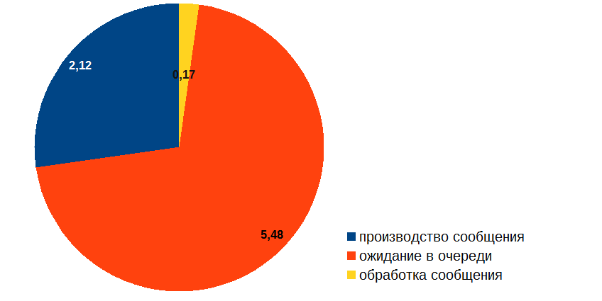
Thus, despite the fact that processing a message takes quite a bit of time, most of all the message is idle in the queue. How can this be? And most importantly: how to deal with it? After all, if the picture above was the result of profiling the usual code, then everything would be obvious: it is necessary to optimize the “red” procedure. But the trouble is that in our case nothing happens in the “red” zone, the message is just waiting in the queue! It is clear that the message processing needs to be optimized (the “yellow” part of the diagram), but questions arise: how can this optimization affect the queue length and where are the guarantees that we can achieve the desired result?

I remembered that queuing theory deals with probabilistic estimates of waiting time in a queue (a subsection of operations research ). At the time, at the university, however, we didn’t go through this, so for some time I had to dive into Wikipedia, PlanetMath and online lectures, from where information about Kendall notation , Little’s law , Erlang formulas , and so on fell from my horn of plenty. dd, etc.

The analytical results of the queuing theory are replete with quite serious mathematics, most of these results were obtained in the XX century. Studying all this is a fascinating occupation, but rather long and laborious. I can not say that I was able to dive at least some deep.

And nevertheless, having run only “on top” of the queuing theory, I found that the main conclusions that can be applied in practice in our case, lie on the surface, require only common sense for their justification and can be depicted on the graph processing time in the system with a queue of server bandwidth, here it is:



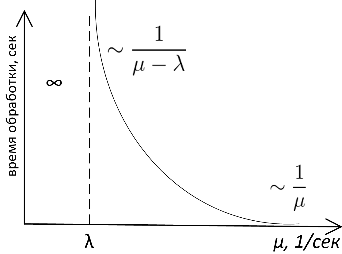
Here

• $$$\ mu$ - server bandwidth (in messages per second)
• $$$\ lambda$ - average frequency of requests (in messages per second)
• The ordinate axis shows the average message processing time.

The exact analytical view of this graph is the subject of a study of the theory of queues, and for queues M / M / 1, M / D / 1, M / D / c, etc. (if you don’t know what it is, see Kendall’s notation ) This curve is described by completely different formulas. However, whatever model the queue is described, the appearance and the asymptotic behavior of this function will be the same. This can be proved by simple reasoning, which we will do.

First, look at the left side of the graph. It is clear that the system will not be stable if $$$\ mu$ (bandwidth) less $$$\ lambda$ (arrival rates): messages for processing come with a greater frequency than we can process, the queue grows indefinitely, and we are in serious trouble. In general, the case $$$\ mu <\ lambda$ - emergency always.

The fact that the graph on the right asymptotically tends to $$$1 / \ mu$ , is also quite simple and does not require in-depth analysis for its proof. If the server is very fast, then we practically do not wait in the queue, and the total time we spend in the system is equal to the time that the server spends processing the message, and this is just $$$1 / \ mu$ .

It’s not immediately obvious that when approaching $$$\ mu$ to $$$\ lambda$ on the right side the waiting time in the queue grows to infinity. In fact: if $$$\ mu = \ lambda$ then this means that the average processing speed of messages is equal to the average speed of receiving messages, and it seems intuitively that in this situation the system should cope. Why is the graph of time versus server performance at point $$$\ lambda$ flies to infinity, and does not behave like this:



But this fact can be established without resorting to serious mathematical analysis! To do this, it is enough to understand that the server, processing messages, can be in two states: 1) it is busy with work 2) it is idle because it has processed all tasks, and new ones have not yet arrived in the queue.

Jobs in the queue come unevenly, where "thicker, where less often": the number of events per unit of time is a random variable, described by the so-called Poisson distribution . If the tasks were rarely run at some time interval and the server was idle, then the time during which it was idle could not be “saved” in order to use it for processing future messages.

Therefore, due to server idle periods, the average speed of event logout from the system will always be less than the peak server bandwidth.

In turn, if the average exit speed is less than the average entry speed, then this leads to an infinite lengthening of the average waiting time in the queue. For queues with a Poisson distribution of events at the input and with a constant or exponential processing time, the expectation value near the saturation point is proportional to

$$

$$\ frac {1} {\ mu- \ lambda}.$$

findings

So, looking at our schedule, we come to the following conclusions.

• Message processing time in the queue system is a server bandwidth function. $$$\ mu$ and average frequency of receipt of messages $$$\ lambda$ , and even simpler: it is a function of the ratio of these quantities $$$\ rho = \ lambda / \ mu$ .
• Designing a system with a queue, you need to estimate the average frequency of arrival of messages. $$$\ lambda$ and lay down server bandwidth $$$\ mu >> \ lambda$ .
• Every system with a queue depending on the ratio $$$\ lambda$ and $$$\ mu$ can be in one of three modes:
  
  
  1. Emergency mode - $$$\ mu \ leq \ lambda$ . The queue and processing time in the system grow indefinitely.
  2. Mode close to saturation: $$$\ mu> \ lambda$ but not by much. In this situation, small changes in server bandwidth greatly affect the performance of the system, both in that and in the other direction. Need to optimize the server! However, even a small optimization can be very beneficial for the entire system. Estimates of the speed of receipt of messages and the bandwidth of our service showed that our system worked just around the “saturation point”.
  3. Mode "almost without waiting in the queue": $$$\ mu >> \ lambda$ . The total time spent in the system is approximately equal to the time that the server spends processing. The need for server optimization is already determined by external factors, such as the contribution of the subsystem with the queue to the total processing time.

Having dealt with these issues, I proceeded to optimize the event handler. Here is the situation in the end:


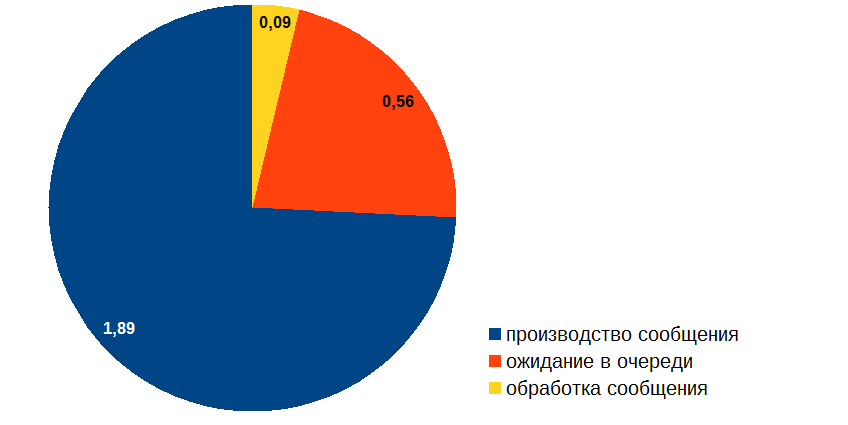
OK, now it is possible to suboptimize the message production time!

I also recommend reading: Principles and techniques for processing queues .