Will Python save from execution?
Good day! When watching action films (movies with well-thought-out dynamic scenes) sometimes creeps in your head: is it real? For example, could a car roll over at low speed, how fast can you swing on a rope without initial speed over the precipice ...

What does physics say to this? Is it interesting to write on paper and then show off a piece of formulas and a couple of vectors? Let's do it safely and visually.
Let's start with the usual mathematical pendulum :
')
We divide the equation into two first order and write in the standard form
And now we boldly feed it to our snake (more about scipy.integrate.odeint , alas, in the original).
In the first year in the laboratory, the mechanics were pendulums, the capabilities of each of them almost exhausted the task to work. Butthere was something wrong with one, because the Oberbec pendulum couldn’t attract the most attention: “What will happen if we do not fix the weights?”
And now, after N years, I saw in the film (the next pirates of the Caribbean) what will happen!
Hmmm, is it really so? To do this, it is enough to write down only two equations, the first of which is written in the rest system of the guide blade, taking into account the portable and Coriolis acceleration.
Where is the weight of the guillotine? As in most tasks without friction, it was right and left of equality, and does not affect anything.
Enjoying the results:
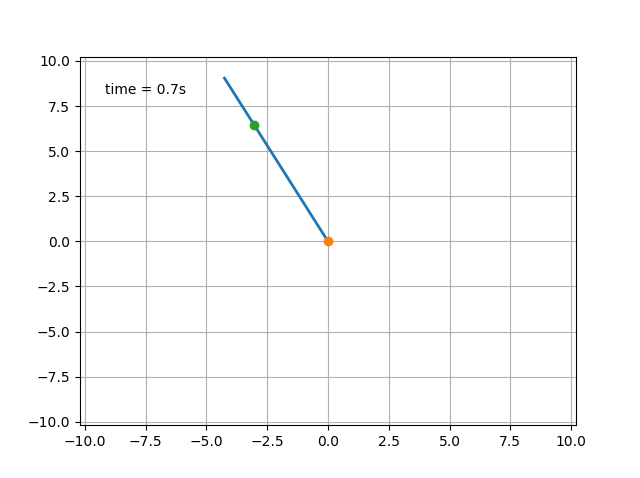
If the initial velocity is high, then this “attraction” is safe after passing through a horizontal position.
PS started digging here .
Having played with the initial parameters (for small angles of deviation from the vertical or small initial angular velocities), one can come to a “flat” understanding of the stability of gyroscopes.
And it is better to be kind and do not fall under the guillotine!
What does physics say to this? Is it interesting to write on paper and then show off a piece of formulas and a couple of vectors? Let's do it safely and visually.
Let's start with the usual mathematical pendulum :
By the way, even if we take the sine as its argument, then experiments with measuring the period of the pendulum give good results for g. But we, in order to admire large angles, must honestly solve the equation, especially if scipy provides such an opportunity.
')
We divide the equation into two first order and write in the standard form
And now we boldly feed it to our snake (more about scipy.integrate.odeint , alas, in the original).
t = linspace(0,15,100) G = 9.8 L = 1.0 def diffeq(state, t): th, w = state return [w, -G/L*sin(th)] dt = 0.05 t = np.arange(0.0, 20, dt) th1 = 179.0 w1 = 0.0 state = np.radians([th1, w1]) y = odeint(diffeq, state, t) In the first year in the laboratory, the mechanics were pendulums, the capabilities of each of them almost exhausted the task to work. But
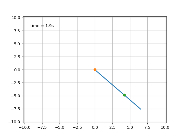
And now, after N years, I saw in the film (the next pirates of the Caribbean) what will happen!
Hmmm, is it really so? To do this, it is enough to write down only two equations, the first of which is written in the rest system of the guide blade, taking into account the portable and Coriolis acceleration.
Where is the weight of the guillotine? As in most tasks without friction, it was right and left of equality, and does not affect anything.
Enjoying the results:
If the initial velocity is high, then this “attraction” is safe after passing through a horizontal position.
import matplotlib.animation as animation from pylab import * from scipy.integrate import * import matplotlib.pyplot as plt t = linspace(0,15,100) G = 9.8 L = 10.0 def derivs(state, t): th, w, r, v = state if 0.<r<L or w**2*r>G*cos(th): return [w, -G/r*sin(th), -v, (-w**2*rG*cos(th)-G*sin(th)-2*w*v)] elif w**2*r<G*cos(th): return [w,-G/r*sin(th),-v, w**2*rG*cos(th)] return [w,-G/r*sin(th), 0,0] dt = 0.01 t = np.arange(0.0, 20, dt) th1 = 180.0 w1 = 50. r1 = L*0.9 v1 = 0.0 state = np.radians([th1, w1]) state = np.append(state, [r1, v1]) y = odeint(derivs, state, t) x1 = L*sin(y[:, 0]) y1 = -L*cos(y[:, 0]) x2 = (y[:,2].clip(min = 0, max = L))*sin(y[:, 0]) y2 = -(y[:,2].clip(min = 0, max = L))*cos(y[:, 0]) fig = plt.figure() ax = fig.add_subplot(111, autoscale_on=False, xlim=(-L-0.2, L+0.2), ylim=(-L-0.2, L+0.2)) ax.grid() line, = ax.plot([], [], '-', lw=2) point, = ax.plot(0,0,'o', lw=2) extra, = ax.plot(x1/L*r1,y1/L*r1,'o', lw=2) time_template = 'time = %.1fs' time_text = ax.text(0.05, 0.9, '', transform=ax.transAxes) def init(): line.set_data([], []) point.set_data(0,0) time_text.set_text('') extra.set_data(x1/L*r1,y1/L*r1) return line, time_text, point, extra def animate(i): thisx = [0, x1[i]] thisy = [0, y1[i]] thisx2 = x2[i] thisy2 = y2[i] point.set_data(thisx[0],thisy[0]) line.set_data(thisx, thisy) time_text.set_text(time_template % (i*dt)) extra.set_data([thisx2,thisy2]) return line, time_text, point, extra ani = animation.FuncAnimation(fig, animate, np.arange(1, len(y)), interval=25, blit=True, init_func=init, repeat = False) show() PS started digging here .
Having played with the initial parameters (for small angles of deviation from the vertical or small initial angular velocities), one can come to a “flat” understanding of the stability of gyroscopes.
And it is better to be kind and do not fall under the guillotine!
Source: https://habr.com/ru/post/332620/
All Articles