Identification of cointegrated pairs of shares in stock markets

The purpose of this article is to share the results of a study to identify cointegrated pairs of stocks that are represented on the Moscow and New York stock exchanges, using the Angle-Granger test.



If we take two stocks with stationary increments , and find them some linear combination (spread), which will be stationary, then such a time series will be called cointegrated. The presence of cointegration gives us the opportunity to hedge shares and build a market neutral strategy. Why is this possible?

The principle on which profit is built

We all know that the price of a stock, regarded as a time series, can change quite significantly. If we make a position in any one paper, in most cases it will be a very risky game, since we will take all the risks associated with its volatility. However, there are such actions, from which it can be expected that, being paired, such series will not move too far from each other. This concept is called long-term dynamic equilibrium.



In the context of stationarity, long-term dynamic equilibrium takes on a more accurate form. If we take the stationary range of the spread, built between two cointegrated papers, it will have the property of returning to the average, that is, with any deviation from a certain equilibrium, it will tend to return back. The market neutral strategy is based on this principle.

')

How in the stock markets to find pairs connected by long-term dynamic equilibrium?

Correlation

The first thought that comes to mind is to calculate the correlation between the two papers and trade pairs with a strong correlation. This approach fails for two reasons.



First, if the price series of two stocks would have an ideal correlation, that is, if they changed in the same direction and in the same proportion, the difference between the rows would be zero, and we would not be able to earn any money, because none of the stocks will ever be too expensive or too cheap.



Secondly, the correlation does not give us enough information about the relationship of the two shares in the long term. For example, take a large and diversified portfolio of stocks. Let these shares also be included in the stock index, and let the weight of shares in the portfolio be determined by their weights in the index. Although the portfolio in the long run should move in accordance with the index, there will be periods when stocks that are in the index, but not in the portfolio, will have unusual price movements. Consequently, the empirical correlations between the portfolio and the index can be rather low for some time. Because of this, in the analysis, we simply discard such a portfolio and lose the opportunity to earn. It follows that correlation is not a good way to identify pairs.



It is better to use cointegration to identify pairs.

Cointegration

Often, to ensure the stationarity of the economic series, we take the difference. This leads to the following definition of integration.



The time series is called the integrated order. $$$k$ and denoted by $$$x_t \ sim I (k)$ if he and his difference to order $$$k-1$ inclusively nonstationary, and its order difference $$$k$ stationary.



We only need the values ​​to get practical results. $$$k = 0$ and $$$k = 1$ . If a $$$k = 0$ then the series itself will be stationary, and for brevity I will further denote such series $$$I (0)$ . For $$$k = 1$ the series will be non-stationary with stationary increments (first-order differences), and for brevity I will further denote such series $$$I (1)$ .



May we have two $$$I (1)$ row, $$$x_t$ and $$$y_t$ . Let, moreover, their linear combination $$$y_t - \ beta x_t$ is an $$$I (0).$ In this case, the rows $$$x_t$ and $$$y_t$ are called cointegrated:

$$

$$\ varepsilon_t = y_t - \ beta x_t \ sim I (0).$$

In essence, cointegration is a regression of non-stationary series. It means that if $$$\ varepsilon_t$ has a zero mean, then this series will rarely deviate far from zero and often cross the zero level. In other words, from time to time, an exact equilibrium or a state close to it will be achieved.

Cointegration of logarithms of prices

We can consider cointegration not only between prices, but also between their logarithms. Unfortunately, cointegration between the logarithms of the prices of two stocks is less obvious and intuitive than just cointegration between the prices of two stocks. However, why is cointegration possible in the case of logarithms?



This is explained by the “efficient market hypothesis”, option pricing model and Ito's lemma. In fact, the effective market hypothesis does not have a strict formalization. This hypothesis suggests that in a liquid market, where the price of an asset will be the result of a balanced spontaneous supply and demand, the current price will accurately reflect all the information that is available to market players. Future changes in price can only be the result of “news”, which by definition is unpredictable, so the best price forecast for any future date is just the price today. In other words, the price today is yesterday's price plus a random item.



The hypothesis of an effective market is connected with the basic pricing model of options. The fundamental assumption of this model is that the price of the underlying asset $$$S$ satisfies the process of geometric Brownian motion (GBM):

$$

$$\ frac {dS} {S} = \ mu dt + \ sigma dW,$$

Where $$$\ mu$ and $$$\ sigma$ - constants, which represent, respectively, the displacement in the price of the asset and the volatility of profitability, and $$$W$ - this is a Wiener process, that is, increments $$$dW$ independent and normally distributed with zero mean and variance $$$dt$ .



To see how the GBM equation is related to the efficient market hypothesis, one needs to apply Ito’s lemma to it. What is it? Assume that the values ​​of a variable $$$x$ obey the stochastic differential equation (SDE)

$$

$$dx = \ mu dt + \ sigma dW,$$

Where $$$W$ Is a Wiener process, and $$$\ mu$ and $$$\ sigma$ - functions that depend on variables $$$x$ and $$$t$ . Assume also that the function $$$f$ depends on variables $$$x$ and $$$t$ and has derivatives $$$\ frac {\ partial f} {\ partial t}$ , $$$\ frac {\ partial f} {\ partial x}$ , $$$\ frac {\ partial ^ 2 f} {\ partial x ^ 2}$ . Lemma Ito argues that this function obeys the equation

$$

$$df = (\ frac {\ partial f} {\ partial t} + \ mu \ frac {\ partial f} {\ partial x} + \ frac {\ sigma ^ 2} {2} \ frac {\ partial ^ 2 f} {\ partial x ^ 2}) dt + \ sigma \ frac {\ partial f} {\ partial x} dW.$$

In essence, Ito's lemma is a formula for changing variables in the CDS, where under certain conditions the function of some CDS is also the CDS.



Let us return to the GBM equation and transform it into

$$

$$dS = \ mu Sdt + \ sigma SdW.$$

Putting $$$f = f (s, t)$ , by Ito's lemma we get:

$$

$$df = (\ frac {\ partial f} {\ partial t} + \ mu S \ frac {\ partial f} {\ partial S} + \ frac {\ sigma ^ 2 S ^ 2} {2} \ frac { \ partial ^ 2 f} {\ partial S ^ 2}) dt + \ sigma S \ frac {\ partial f} {\ partial S} dW.$$

We introduce a function $$$f (S) = \ ln ⁡S$ . Insofar as

$$

$$\ frac {\ partial \ ln ⁡S} {\ partial S} = \ frac {1} {S}, \ frac {\ partial ^ 2 \ ln ⁡S} {\ partial S ^ 2} = - \ frac { 1} {S ^ 2}, \ frac {\ partial \ ln ⁡S} {\ partial t} = 0,$$

we get:

$$$$ display $$ d \ ln ⁡S = (\ frac {\ partial \ ln S} {\ partial t} + \ mu S \ frac {\ partial \ ln ⁡S} {\ partial S} + \ frac { \ sigma ^ 2 S ^ 2} {2} \ frac {\ partial ^ 2 \ ln ⁡S} {\ partial S ^ 2}) dt + \ sigma S \ frac {\ partial \ ln ⁡S} {\ partial S } dW = \\ = (0 + \ mu S \ frac {1} {S} - \ frac {\ sigma ^ 2 S ^ 2} {2} \ frac {1} {S ^ 2}) dt + \ sigma S \ frac {1} {S} dW = (\ mu - \ frac {\ sigma ^ 2} {2}) dt + \ sigma dW. $$ display $$

The equation

$$

$$d \ ln ⁡S = (\ mu - \ frac {\ sigma ^ 2} {2}) dt + \ sigma dW$$

can be rewritten in discrete form

$$

$$\ Delta \ ln S_t = c + \ varepsilon_t,$$

Where $$$c = \ mu - \ sigma ^ 2/2$ , but $$$\ varepsilon_t \ sim NID (0, \ sigma ^ 2)$ so there is a process $$$\ varepsilon_t$ not just stationary, but a white noise. The concept of a stationary process is broader than white noise, and it differs in that a stationary process has a constant expectation, but it does not have to be zero, as is the case with white noise.



The discrete version of the equation given above can, in turn, be written as:

$$

$$\ ln⁡ S_t = c + \ ln S_ {t-1} + \ varepsilon_t.$$

This equation is a random walk (RW) model that is commonly used to simulate price logarithms in efficient financial markets, and is an example $$$I (1)$ process. Thus, cointegration can also refer to the logarithms of stock prices.



Despite the fact that some skeptics (in particular, I) may doubt the adequacy of the description of the stock price by the GBM equation and, therefore, the possibility of cointegration between price logarithms, empirical data successfully dispel this skepticism. I checked: if the prices are cointegrated, then their logarithms are cointegrated.

Cointegration testing

The first method of testing cointegration came up with Robert Angle and Clive Granger. In 2003, they received the Nobel Prize in Economics for developing a cointegration method for analyzing time series. They described it 15 years before the prize, in 1987 in the article “Cointegration and error correction: representation, estimation and testing”.



Conceptually, in order to determine from existing observations whether time series are $$$x_t$ and $$$y_t$ cointegrated, we need to test the null hypothesis $$$H_0: \ varepsilon_t \ sim I (1)$ the absence of cointegration between the rows $$$x_t$ and $$$y_t$ against alternative hypothesis $$$H_0: \ varepsilon_t \ sim I (0)$ . If the null hypothesis is rejected, then cointegration is recognized.



The original test for cointegration received the name of the test Angle-Granger in honor of its founders. It is a two-step process preceded by a check. $$$x_t$ and $$$y_t$ on first-order integrability, $$$x_t \ sim I (1)$ and $$$y_t \ sim I (1)$ . We discussed this in detail in the article on stationary increments . In fact, it describes all the preparatory work that needs to be done before proceeding directly to the Angle-Granger test. Let's say we did it.



Rows $$$x_t$ and $$$y_t$ are co-integrated if their spread $$$y_t - \ beta x_t \ sim I (0)$ , that is, is stationary. The first step in the Engle-Granger test is to obtain a consistent assessment. $$$\ hat {\ beta}$ . This is done using the OLS (least squares method) for linear regression to the equation $$$y_t = \ beta x_t + \ varepsilon_t$ . The second step is to check for stationary residues $$$\ varepsilon_t$ obtained by OLS-estimation of the cointegration equation.



Usually we test stationarity with the Dickie-Fuller test. However, in 1990, Phillips and Uliaris in the article "Asymptotic properties of residual based tests for cointegration" showed that a series of $$$\ varepsilon_t$ Dicky-Fuller's test cannot be used.



The fact is that the OLS “chooses” the residues so that they have the smallest possible variation, therefore, even if the variables are not cointegrated, the OLS makes the residues “similar” to the stationary ones. Because of this, when using the Dickey-Fuller test, the hypothesis of non-stationarity is rejected too often and, accordingly, the hypothesis of cointegration is mistakenly accepted.



If we study the authors' article, we will see that in the appendix they give tables with critical values, however they turned out to be rather inaccurate. Later, in 1991, Engle and Granger published the Long-Run Economic Relationship book. In her 13th chapter, entitled “Critical value for cointegration tests,” McKinnon gave refined asymptotic critical values. $$$t$ - statistics that were obtained by simulation and are suitable for this case.



In 1993, McKinnon, together with Davidson, published his book “Estimation and Inference in Econometrics”, where they also gave updated critical values. Thus, if $$$\ varepsilon_t \ sim I (0)$ (residues are stationary), then $$$y_t - \ beta x_t \ sim I (0)$ (the spread is also stationary), which means that there is a cointegration between $$$x_t$ and $$$y_t$ .



In general, the Angle-Granger method is reduced to:

1. assessment $$$\ beta$ using OLS;
2. spread calculation $$$\ varepsilon_t = y_t - \ beta x_t$ and testing $$$\ varepsilon_t$ on stationarity with the help of specified critical values.

In standard packages such as Matlab, this test has already been written, let's use it.

MATLAB cointegration testing

So, we have two rows of stock prices, $$$x_t$ and $$$y_t$ . we want to $$$x_t$ and $$$y_t$ were co-integrated, that is, to spread $$$\ varepsilon_t = y_t - \ beta x_t$ was stationary. If we want to get a stationary series with zero mean, we can include a constant in the equation, so the spread will look like $$$\ varepsilon_t = y_t - \ beta x_t - \ alpha$ .



Let's start with the results obtained on the Moscow Stock Exchange, which I described in the article about stationary increments . There I found five $$$I (1)$ rows. We will make of them all sorts of combinations and check for cointegration with the help of Angle Granger's test.



First, we will select from the Microsoft SQL Server database, in which I store the stock price values ​​we needed from the Moscow Stock Exchange and the papers we need and import them as an array:

conn = database.ODBCConnection('uXXXXXX.mssql.masterhost.ru', 'uXXXXXX', 'XXXXXXXXXX'); curs = exec(conn, 'SELECT ALL PriceId, StockId, Date, Price FROM StockPrices WHERE StockId IN (52, 55, 67, 75, 162) AND Date >= ''2016-01-01 00:00:00.000'' AND Date < ''2017-01-01 00:00:00.000'''); curs = fetch(curs); data = curs.Data sqlquery = 'SELECT ALL StockId, ShortName, Code FROM Stocks WHERE StockId IN (52, 55, 67, 75, 162)'; curs = exec(conn, sqlquery); curs = fetch(curs); names = curs.Data close(conn); 

In this array for four out of five stocks there is data from January for 252 trading days. However, for one of the shares, deals began to be made only in February, so the data is only for 215 trading days. It is critically important for us that all stocks have an array of prices of the same length, so in such situations we have two options.



The first option is to exclude a stock with a short array of prices from the experiment and use the maximum number of price measurements in order to get more accurate results. The second option is to donate part of the data and include all the shares for the sake of greater practicality. I conducted both experiments, and in this case there was no difference in the results, so let's just cut off the January data:

 dates = unique(datetime(data(:,3))); % Cut dates array until price of stock with StockId=67 is not empty. dates(1:37,:) = []; prices = zeros(length(dates),length(names)); for i = 1:length(names) % Indexes with current stock's data indexes = find(cell2mat(data(:,2)) == cell2mat(names(i,1))); if length(indexes) == 252 indexes(1:37,:) = []; end for j=1:length(dates) % Fill prices according to date prices(j,i) = cell2mat(data(indexes(j),4)); end end 

The Angle-Granger test is performed using the egcitest function, which takes as its input an array of time series, in this case the size $$$n \ times 2$ where $$$n$ - number of trading days. At the output, the function returns a logical value of 1 if the null hypothesis is rejected in favor of the alternative, and 0 otherwise.



The next task we need to solve is what action to take for $$$x_t$ and which - for $$$y_t$ . In an amicable way, one should try both, and then compare test statistics. In most cases, there will be both direct and reverse regression. Let's start with the case when $$$x_t <y_t$ .



We make all possible pairs of five identified $$$I (1)$ series and perform the Engle-Granger test for both regression with a free member (by default) or without it (given by the 'creg' argument with a value of 'nc'):

 isCoint = zeros(length(nchoosek(names(:,1),2)), 3); k=1; for i=1:length(names) for j=i+1:length(names) if mean(prices(:,i)) < mean(prices(:,j)) isCoint(k,1) = cell2mat(names(j,1)); isCoint(k,2) = cell2mat(names(i,1)); testPrices(:,1) = prices(:,j); testPrices(:,2) = prices(:,i); else isCoint(k,1) = cell2mat(names(i,1)); isCoint(k,2) = cell2mat(names(j,1)); testPrices(:,1) = prices(:,i); testPrices(:,2) = prices(:,j); end isCoint(k,3) = egcitest(testPrices); isCoint(k,4) = egcitest(testPrices, 'creg', 'nc'); k = k + 1; end end 

In the case of regression with a free member, the program twice rejects the null hypothesis in favor of an alternative model, identifying cointegrated pairs of stocks with tickers (NKHP, VTRS), (NKHP, ZHIV). In the case of a regression without a free member, the program once rejects the null hypothesis in favor of the alternative, identifying a cointegrated pair of shares with tickers (VSYDP, NKHP).



In case of reverse regression ( $$$y_t <x_t$ ) with a free member, the program twice rejects the null hypothesis in favor of an alternative model, identifying cointegrated pairs of shares with tickers (VTRS, NKHP), (ZHIV, NKHP). In the case of regression without a free member, the program four times rejects the null hypothesis in favor of the alternative, identifying cointegrated pairs of shares with tickers (GRNT, VTRS), (GRNT, VSYDP), (GRNT, ZHIV), (GRNT, NKHP).



Let's estimate the values $$$\ beta$ and $$$\ alpha$ , which can be obtained as return values ​​of the egcitest function, and draw a spread:

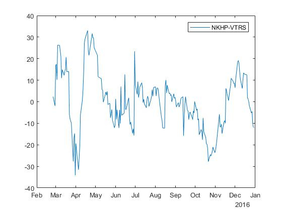
 % NKHP and VTRS indexY = 5; indexX = 1; testPrices(:,1) = prices(:,indexY); testPrices(:,2) = prices(:,indexX); [h,pValue,stat,cValue,reg1,reg2] = egcitest(testPrices); alpha = reg1.coeff(1); beta = reg1.coeff(2); spread = reg1.res; plot(dates,spread) legend(strcat(names(indexY,3),'-',names(indexX,3))); 

For stocks with tickers NKHP and VTRS, we obtain a spread with coefficients $$$\ beta = $ 37.552$ and $$$\ alpha = $ 197.439$ :



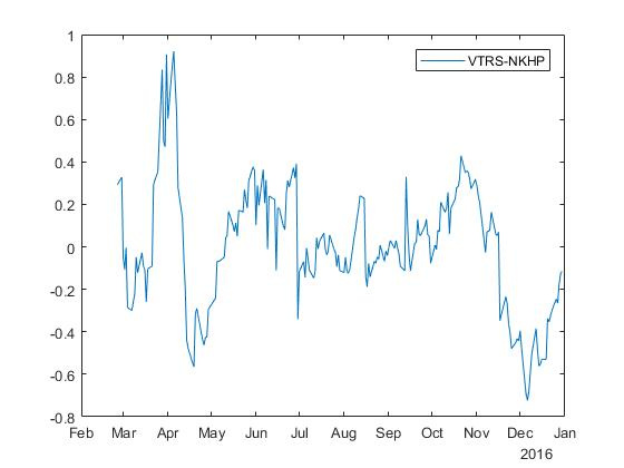
For reverse regression, we get a “mirror” spread with coefficients $$$\ beta = $ 0.085$ and $$$\ alpha = -3,0064$ :



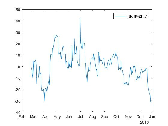
For stocks with tickers NKHP and ZHIV, we obtain a spread with coefficients $$$\ beta = $ 3.352$ and $$$\ alpha = $ 239.347$ :



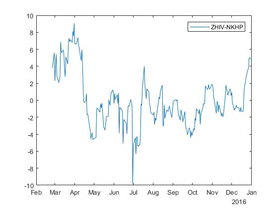
For reverse regression, we obtain a spread with coefficients $$$\ beta = 0.2194$ and $$$\ alpha = -49,6077$ :



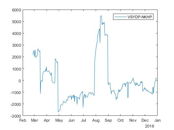
For stocks with tickers VSYDP and NKHP, we obtain a spread with a coefficient $$$\ beta = $ 35.652$ :





Similar experiments were carried out for the shares of the New York Stock Exchange (NYSE). As a result, 158 cointegrated pairs were obtained for direct regression in the case of regression with a free member and 130 cointegrated pairs in the case of regression without a free member. For backward regression, 170 cointegrated pairs were obtained in the case of regression with a free member and 144 cointegrated pairs in the case of regression without a free member.

Regression Statistics

Let's look at the regression statistics of cointegrated regression for a pair (NKHP, VTRS).

Statistics	Direct regression	Inverse regression
Coefficients	$$$\ beta = $ 37.552$ , $$$\ alpha = $ 197.439$	$$$\ beta = $ 0.085$ , $$$\ alpha = -3,0064$
Test statistics	$$$t_ {calc} = -3.7562$ , $$$t_ {crit} = -3.3654$	$$$t_ {calc} = -3,5906$ , $$$t_ {crit} = -3.3654$
$$$t$ -statistics	$$$t_ \ beta = $ 21.975$ , $$$t_ \ alpha = 53.3845$	$$$t_ \ beta = $ 21.975$ , $$$t_ \ alpha = -12,8953$
$$$F$ -statistics	482,9196	482,9196
Statistics of Durbin-Watson	0.2548	0,2203
Coefficient of determination	0,6939	0,6939
Corrected coefficient of determination	0,6925	0,6925
Akaike Information Criterion	1726.5	88,8336
Schwarz's Baes information criterion	1733.2	95,5748
Hannan-Quinn Information Criterion	1729.2	91.5574

Test statistics in both direct and inverse regression tells us that the variable $$$\ beta$ in this case, insignificant ( $$$t_ {calc} <t_ {crit}$ ). This means that the price may be slightly exogenous, even though the variables are cointegrated.



In order to apply the Student’s criterion and the Fisher criterion, it is necessary that the statistics have a normal distribution. In our case, the statistics has a distribution similar to what Dickie and Fuller established (I also wrote about it in the article about stationary increments ), therefore the calculated values ​​of these statistics will be quite large and nothing meaningful will tell us.



Durbin-Watson statistics are acceptable (with positive autocorrelation, the statistics tend to zero). In the case of reverse regression, it is slightly better than in the case of direct.



The coefficient of determination is acceptable (for acceptable models it is assumed that the coefficient of determination should be at least at least 50%). Judging by this criterion, there is no difference between direct and reverse regression.



Judging by the information criteria, the inverse regression greatly benefits the direct (it is believed that the model with the lowest criterion value will be best).



Look at the regression statistics of the cointegrated regression for the pair (NKHP, ZHIV).

Statistics	Direct regression	Inverse regression
Coefficients	$$$\ beta = $ 3.352$ and $$$\ alpha = $ 239.347$	$$$\ beta = 0.2194$ and $$$\ alpha = -49,6077$
Test statistics	$$$t_ {calc} = -3,4762$ , $$$t_ {crit} = -3.3654$	$$$t_ {calc} = -3.3878$ , $$$t_ {crit} = -3.3654$
$$$t$ -statistics	$$$t_ \ beta = $ 24.344$ , $$$t_ \ alpha = $ 137.97$	$$$t_ \ beta = $ 24.344$ , $$$t_ \ alpha = -19,8524$
$$$F$ -statistics	592,652	592,652
Statistics of Durbin-Watson	0.2614	0,2104
Coefficient of determination	0.7356	0.7356
Corrected coefficient of determination	0.7344	0.7344
Akaike Information Criterion	1695	1108,8
Schwarz's Baes information criterion	1701.7	1115,5
Hannan-Quinn Information Criterion	1697.7	1111.5

Test statistics in both direct and inverse regression tells us that the variable $$$\ beta$ in this case, insignificant. Durbin-Watson statistics are acceptable, in the case of reverse regression, slightly better than in the case of direct. The coefficient of determination is acceptable, there is no difference between direct and reverse regression. According to the information criteria, the inverse regression is slightly better than the direct one.



Coagulation regression statistics for the pair (VSYDP, NKHP).

Statistics	Direct regression
Coefficients	$$$\ beta = $ 35.652$
Test statistics	$$$t_ {calc} = -2,8339$ , $$$t_ {crit} = -2,7761$
$$$t$ -statistics	82.5035
$$$F$ -statistics	$$$\ infty$
Statistics of Durbin-Watson	0.1305
Coefficient of determination	0,1928
Corrected coefficient of determination	0,1928
Akaike Information Criterion	3823,8
Schwarz's Baes information criterion	3827.1
Hannan-Quinn Information Criterion	3825.1

Variable $$$\ beta$ judging by the test statistics, again insignificant. Fisher criterion flew into space. Durbin-Watson statistics are acceptable. The coefficient of determination is small, so the model is considered bad.

findings

There are a sufficient number of cointegrated shares in stock markets, that is, such that their spread is a stationary process. The presence of such pairs provides the basis for further research and a stable profit, but we'll talk about specific strategies next time.

What to read on the topic?

Robert F. Engle, C.W.J. Granger. Cointegration and error correction: presentation, evaluation and testing // Applied Econometrics. - 2015. - 39 (3). - p. 107-135.



This is a translation of the original article by the authors of 1987; the definition of cointegration is described in more detail there. You can also continue to read Magnus, whom I recommended in the article on stationary increments , there is also a section on cointegration.



UPD. Analytics on cointegrated couples for 2017 on the Moscow Stock Exchange .