Annealing and freezing: two fresh ideas on how to accelerate the learning of deep networks.
This post outlines two recently published ideas on how to speed up the learning process of deep neural networks while increasing prediction accuracy. The proposed (by different authors) methods are orthogonal to each other, and can be used together and separately. The methods proposed here are simple to understand and implement. Actually, links to original publications:
1. Ensemble of pictures: many models for the price of one
Ordinary ensembles of models
Ensembles are groups of models used collectively for prediction. The idea is simple: train several models with different hyperparameters, and average their predictions when testing. This technique gives a noticeable increase in the accuracy of the prediction; most winners of machine learning competitions
')
So what's the problem?
Training N models will require N times more time than training a single model.
SGD Mechanics
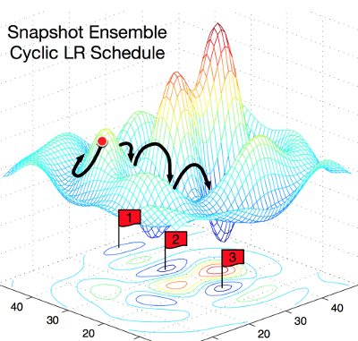
Stochastic Gradient Descent (SGD) is a greedy algorithm. It moves in the parameter space in the direction of the greatest gradient. At the same time, there is one key parameter: learning speed. If the learning rate is too high, SGD ignores the narrow valleys in the relief of the hyperplane of parameters (minima) and jumps over them like a tank through trenches. On the other hand, if the learning rate is low, SGD falls into one of the local minima and cannot get out of it.
However, it is possible to pull the SGD from the local minimum by increasing the learning rate.
Watching hands ...
The authors of the article use this controlled parameter SGD to roll into a local minimum and exit from there. Different local minima can give the same percentage of errors when testing, but the specific errors for each local minimum will be different !
This picture explains the concept very clearly. The left shows how a normal SGD works, trying to find a local minimum. Right: SGD fails to the first local minimum, takes a snapshot of the trained model, then selects the SGD from the local minimum and looks for the next one. So you get three local minima with the same percentage of errors, but different error characteristics.

What does an ensemble consist of?
The authors exploit the property of local minima to reflect different “points of view” on model predictions. Every time when SGD reaches a local minimum, they keep a snapshot of the model, of which they will form an ensemble during testing.
Cyclic cosine annealing
To automatically decide when to dive into a local minimum, and when to leave it, the authors use the learning speed annealing function:

The formula looks cumbersome, but is actually quite simple. Authors use monotonically decreasing function. Alpha - the new value of learning speed. Alpha zero is the previous value. T is the total number of iterations that you plan to use (the size of the batch is X the number of epochs). M - the number of shots of the model you want to receive (ensemble size).
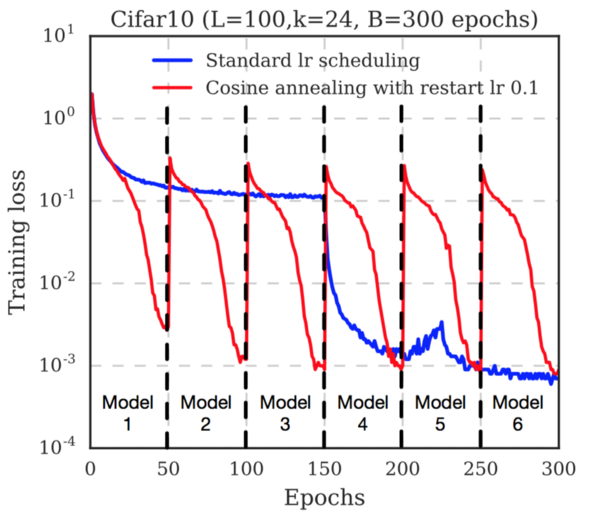
Notice how quickly the loss function drops before saving each shot. This is because the learning rate is continuously decreasing . After saving the snapshot, the learning speed is restored (the authors use a level of 0.1). This deduces the trajectory of the gradient descent from the local minimum, and the search for a new minimum begins.
Conclusion
The authors present test results on several datasets (Cifar 10, Cifar 100, SVHN, Tiny IMageNet) and several popular neural network architectures (ResNet-110, Wide-ResNet-32, DenseNet-40, DenseNet-100). In all cases, an ensemble trained by the proposed method showed the lowest percentage of errors.
Thus, a useful strategy has been proposed for obtaining an increase in accuracy without additional computational costs when training models. On the effect of various parameters, such as T and M on performance, see the original article.
2. Freezing: acceleration of learning by successive freezing of layers.
The authors of the article demonstrated the acceleration of learning by freezing layers without loss of prediction accuracy.
What does freezing layers mean?
Freezing the layer prevents changes in the weights of the layer during training. This technique is often used in transfer learning, when the base model trained in another dataset is frozen.
How does freezing affect model speed?
If you do not want to change the weight of the layer, the reverse passage through this layer can be completely excluded. This seriously speeds up the calculation process. For example, if half the layers in your model are frozen, it will take half as many calculations to train the model.
On the other hand, you still need to train the model, so if you freeze the layers too early, the model will give inaccurate predictions.
What is the novelty?
The authors showed a way to freeze the layers one by one as early as possible, optimizing the learning time by eliminating back passes. At the beginning, the model is fully trained as usual. After several iterations, the first layer of the model is frozen, and the remaining layers continue to be trained. After a few more iterations, the next layer is frozen, and so on.
(Again) annealing learning speed
The authors used annealing learning rate. An important difference between their approach: the learning rate varies from layer to layer , and not for the entire model. They used the following expression:

Here, alpha is the learning rate, t is the iteration number, i is the layer number in the model.
Note that since the first layer of the model will be frozen first, its training will last the least amount of cycles. To compensate for this, the authors scaled the initial learning rate for each layer:

As a result, the authors achieved a 20% acceleration of learning due to a 3% decrease in accuracy , or a 15% acceleration without reducing the prediction accuracy .
However, the proposed method does not work well with models that do not use layer skips (such as VGG-16). In such networks, neither acceleration nor an effect on the prediction accuracy was found.
Source: https://habr.com/ru/post/332534/
All Articles