Automata programming. Part 2. State and transition diagrams
In the first article I gave an example of automaton programming from the general to the particular, or rather, constructive decomposition . The next design stage, the study of the resulting modules. But first, I will show you what automata are from a mathematical and practical point of view. The basis of automata is a model describing the process occurring in time, called a state diagram, and it is impossible to imagine automaton programming without this essence. Why this is so considered in today's article.
Table of contents.
Specialists lead a fairly extensive classification of automata: deterministic and non-deterministic, finite and infinite, Miles and Mura, synchronous and asynchronous, etc. However, from the user's point of view, this is just the same as if a person wanted to decide for himself whether he needed a personal car in the megalopolis, and they would tell him about the number of cylinders and the injector.
')
As a promoter, I note that from the point of view of use, automata fall into two related categories:
The relationship between these approaches is easy to illustrate:
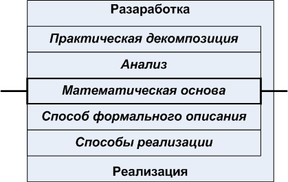
Figure 1. Machine design and machine implementation
As far as it becomes clear from communication with colleagues, there is a category of formalists, people considering automata as:
Obviously, such an approach narrows the space of opportunities that are opened up due to the automata-oriented paradigm, and such an attitude towards automata can be explained only by the lack of popular science material that is fixable.
What I want to use machines for is the simplicity and at the same time the depth of design . In the previous part, it was shown that the automata-oriented design of modules is based on splitting a task into an operational automaton ( OA ) and a control automaton ( UA ), and the operating automaton in turn can be re-divided into a lower-level operational automaton and its controlling automaton .
An operating machine is a semi-finished product that can optimally perform some action, but at the same time it “doesn’t care” when to perform this action and with what parameters. The operating machine can do this with any valid parameters. An excellent example of an ALU operating machine.
In turn, the parametrization and launching of the operating automaton falls on the shoulders of the controlling automaton. The multistage fragmentation makes it possible to avoid obtaining a complex controlling automaton with not obvious, though iron logic, replacing it with several simple controlling automata with the most clear operation.
In this case, the implementation of the control automaton may not be automaton at all, or it may be automaton, but without attributes such as: states rolled up into separate functions, tables of signals and corresponding transitions. And finally, I note that any program is an automatic machine, and yet not all programs are automatically implemented.
But in this case, what is meant by an automatically implemented program?
The main attribute of an automatically implemented program is:
This definition, so to speak, is an invariant, the embodiment of which may be different. In the section Ways to implement automaton programs, we consider a number of examples that illustrate what has been said, but in general the essence is clear.
Now there is a clear criterion by which we assign programs to automatically implemented programs, but someone will ask: what is the trick of the automatic implementation, why in some cases is it more valuable?
The main thing that distinguishes the auto-implemented algorithms from the implemented ones is non-automated lies in the sphere of our psyche, or rather, how we think. As a colleague pointedly noted:
The behavior of an analytical function can be represented as a table or a graph: there is something at the input and there is a one-to-one correspondence at the output. However, most digital devices are such that using analytical functions as bricks, as a result, we still get a program whose behavior depends on the internal state. That is, the use of analytical functions does not solve the problem of "understanding", moving it to another level!
In order to illustrate the term “comprehensibility” and features of human thinking, I propose to consider how the same abstract algorithm, implemented automatically and non-automaticly, is written.
but)
b)
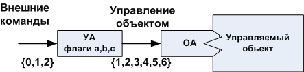
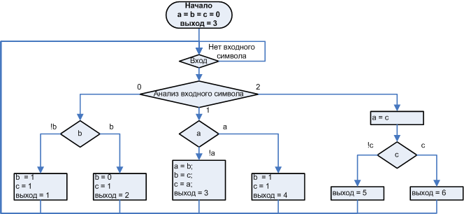
Figure 2. A generalized example of a control device (a) and a graph diagram describing the operation of this device (b).
A certain program is designed to control a certain device. As shown in Fig. 2a, the non-specified OA, which is controlled by the UA, which is shown in Fig. 2, controls the “hardware” directly. 2 (b). The UA processes external commands, conventionally denoted by the {0,1,2} character set, and translates them into a set of microinstructions controlling the operation machine. By microinstructions, I mean a set of commands that is necessary for obtaining an effect. Each set of microinstructions is conditionally denoted by the symbol {1,2,3,4,5,6}. Flags {a, b, c} of the controlling machine monitor the state of the managed object , and, accordingly, determine the processing modes of the input command.
Since this is a digital device with memory, the algorithm described in Fig. 2 is actually an automaton, despite the fact that the implementation of the algorithm is not automatic. This leads to the fact that there are no explicitly selected states in it , with the result that the current state is implicitly determined by flags. In this case, the description of the program by the graph scheme itself does not contradict the automaton principle, an automaton-implemented program can be described by a graph scheme, there will be such an example. The main hitch connected with the graph-scheme is low understanding of the program of the described HS from the point of view of the dynamic, i.e. proceeding in time process.
This is what I mean: this is a very simple example, but it is not possible to unequivocally say which output signal will correspond to the input signal 0, because it will depend on the state of the flags, or rather the flag b, which in turn depends on what was at the entrance earlier. It is also not easy to tell straight away which output sequence will correspond to the input sequence: 2,1,0,2,1,0. To do this, you must actually run the algorithm.
In order to give a complete correspondence of the input and output signals, that is, to describe the function in the form of a table, it will be necessary to perform a total test, and, moreover, the result will be obtained in the form of two-signal sequences, in which various input combinations are iterated.
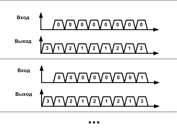
Figure 3. Timing diagram - a way to describe the behavior of systems with memory.
Since the three binary flags allow us to track no more (but possibly no less) of the 8 preceding characters, then for the alphabet of 3 input symbols, to describe all possible options we need to bring 6561 diagrams, the so-called power of the product of the set of input signals and the set of states with increasing number of states and the size of the alphabet of input signals grows geometrically.
Automaton implementation of the program allows you to describe it using the state diagram , and the state diagram and transitions provide a radically different approach to the analysis of dynamic systems with memory. We construct an automaton that implements the algorithm depicted in Fig. 2b (I will not specify how, this is a topic for another conversation), and which is described by a state diagram and transitions depicted in Fig. 4. The state name on the diagram coincides with the output symbol when the automaton in this condition.

Figure 4. State and transition diagrams corresponding to the algorithm shown in Figure 2.
Using this diagram is very convenient, since only input symbols affect transitions, there are no additional conditions. In other words, to analyze the reaction to the input symbol for the implementation of Fig. 2, you need to have the current state of the flags before your eyes, in each iteration a new one, and in order to analyze the behavior of the device implemented as shown in Fig. 4, nothing is needed except this diagram.
This is an important advantage of the automaton approach, called:
The human brain is designed so that it is easier to work with a table of numbers than if the same table is shown one digit at a time. In the first case, a person is able to identify complex patterns, in the second one can hardly determine any pattern, except for the simplest ones, even if you scroll through the table cyclically.
Consider an example, let us have a sequence of commands
You must admit that each of the actions is distinguished by its simplicity of purpose. However, not completing all the actions can not say that we will succeed. The result of this algorithm is shown in Fig. 5 a

a) b)
Figure 5. The result of executing a sequence of commands (a), and the result of executing the same sequence, if an error is made (b).
At the same time, make a mistake in the calculations, and specify, for example, in the first operator of the second line instead of (1, -3) the value of (2, -3) the result of the work would be different (5 b), but looking at the text of the program of this can not understand. And this is a simple case when the result can be seen immediately after execution. If we saw the result as a single line at each moment of time, or dealt not with graphics, but with numbers, our error would not be so obvious.
This is a complex information for the human brain, called a dynamic process, as a sequence of actions (in the example, separate lines), resulting in the imposition of some intended result (in the example of the figure).
A good example of looking at dynamic processes outside the time axis is the analysis of signals in the frequency domain. Consider the signal in Fig. 6. In some ways it can be compared with the time diagram of the automaton. This is also a sequence of actions: the signal crossed 0, went up, reached a maximum, went down, crossed 0 again.
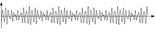
Figure 6. Signal graph, analogue of the timing diagram for automata.
Obviously, this is a periodic signal, one can even guess that it consists of several sinusoids, but it is difficult for us to say from which ones.
At the same time, the spectrum directly gives us an idea of the structure of the signal.

Figure 7. The spectrum of the signal shown in Figure 6.
The spectrum can be compared with the automaton diagram in the following respect: it contains a static description of what underlies the process that takes place in time . Both the spectrum and the state and transition diagram make it possible to analyze the process outside the time axis, encompassing it as a whole, and not as a sequence of steps.
The state and transition diagram as a rigorous mathematical category allows for in-depth analysis.
Let us analyze the process described by the diagram of states and transitions in Fig. 5. For this we need the concept of an isomorphic automaton. Isomorphic automata is a mathematical term for automata, which are actually the same automaton with renamed states and / or signals.
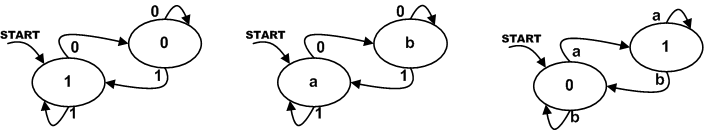
Figure 8. Isomorphic automata.
From the conditions of the problem, it follows that we know nothing about the processes that are simulated by the algorithm in Fig. 2 b. Nevertheless, the analysis given in fig. 4 diagrams allows you to select two very similar clusters, switching between which is performed mainly by signal 0.
We construct an automaton isomorphic to the original, but in which the state numbers have been renamed as shown in Fig. 9 and outlined on it the indicated clusters. In the cluster with the states 4,5,6 in brackets the identical states of the first cluster are indicated.
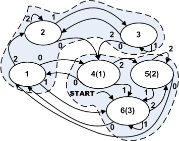
Figure 9. An automaton isomorphic to that depicted in Figure 4
We decompose (we divide) the initial automaton into two parallel automata, as shown in Fig. ten.
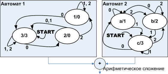
Figure 10. Parallel decomposition of the automaton shown in Figure 9.
The output symbol of each of the machines is given after the slash after the name of the state. The output symbols of the received automata are arithmetically added, giving the output symbols from 1 to 6, which completely correspond to the symbols at the output of the original automaton with the same input data. Such a combination of automata is called a parallel composition.
Pay attention to Automatic 2 . Whatever state it is in, input symbol 0 causes appearance of symbol 1, input symbol 1 leads to the appearance of symbol 3, and symbol 2 to the appearance of symbol 2. That is, in fact, this is a combinational circuit, an array of output symbols, and the array index is the character at the input. Figure machine as shown in Fig. eleven
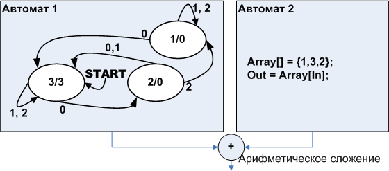
Figure 11. An automaton equivalent to the automaton shown in fig. ten
Since the output symbols we encoded a certain set of microinstructions, it may seem that arithmetic transformations are inappropriate here, however, if you look at the problem through the eyes of a mathematician and imagine that we have an array of implemented microinstructions, in which each microinstruction has an index, in this case the correctness is Our transformations are beyond doubt.
I would like to emphasize that since the characters 0,1,2 at the input and the characters 1,2,3 at the output belong to different alphabets, then you cannot just take and give the character 1 from the output back to the input. However, there may be such automata in which the input and output symbols belong to the same alphabet and in this case, the output symbols of the automaton can be fed to its input. This is called composition with feedback . Section 4.7 is devoted to such compositions.
From the condition of the problem, the nature of the object, which is modeled by the algorithm, was not known.
rice 2 b, and nevertheless, analyzing and decomposing automata, we established that the basis of the simulated phenomenon is actually two independent processes that contribute to the final result. And although in the case of an abstract example, this does not give anything but an interesting observation, in the case of a specific task, the above analysis may reveal non-obvious aspects of the modeled phenomenon, therefore it is interesting not only from the point of view of programming, but also from an engineering point of view. For an engineer, an understanding of the processes underlying the phenomenon can correct the view on the device being developed and get an original technical solution that beats the essence.
The considered example involves another important and useful property of automata, the concept of equivalent automata . The fact is that there can be arbitrarily many automata with different numbers of states (i.e., we are not talking about isomorphic automata) that will give the same response to the same input sequence. Accordingly, if you put them in the “black box”, you will not be able to distinguish them by supplying different sequences to the input and analyzing the response.
Some automata will be more “wasteful” in terms of the number of internal states, while others are more “economical.” Among the entire set of equivalent automata there will be an automaton with the minimum possible number of states, and it is called the minimal automaton . Moreover, there are algorithmic methods for obtaining from any automaton an equivalent minimal one. This property in particular means that when drawing up a diagram of states and transitions one should not strive to minimize the number of states, but one should achieve the most clear and complete picture. And although understanding and simplicity of implementation are often related, it may turn out that it is clearer to present the result as a pair of automata as in our example. After that, using mathematical algorithms, you can find the equivalent minimum automaton.
Since I have no intention to consider in this article the theory of automata, I will briefly list the basic mathematical operations that can be performed on automata: composition, decomposition, minimization, obtaining an automaton from a microprogram, obtaining an automaton-based microprogram, algebraic operations on automata (addition, comparison of automata ), construction of a simulating automaton, etc. Theoretical substantiations and methods for performing these transformations can be found, for example, here .
Summarize today's part. A characteristic feature of non-automatic programming is that the state of the program at any given time is described not only by the program counter, but also by a certain number of internal flags. The term state in the non-automatic style of programs is a kind of non-formalizable concept, meaning roughly that the program performs all the actions that TK requires. And nevertheless, as it was shown above, even with the non-automatic style of the program, mathematically it is an automaton. It has states in a mathematical sense , but these states are not described anywhere. It is not known how many of them and what the relationship between them. Adding each new binary flag increases the number of possible states geometrically. Many new states will be unattainable states in which the program should never get under any conditions, but since in this case we do not explicitly select the next state, but it turns out as a superposition of all flags, with the wrong logic at least one of the flags can jumping into forbidden states and there is no indicator that would demonstrate this. When we deal with flags that are actively changing, and the path of the program is tortuous and goes through many branches, until all options for all possible input symbols are tested, we can only believe that after the twentieth iteration the program will in the state that we expect.
In the case of an automaton implementation, the state is a mathematical category. At each moment of time it is uniquely determined, in particular, by a program counter. We ourselves set the set of states that is needed to solve the control problem, and for each state we explicitly choose, based on needs, which state will be next if the X or Y command arrives . If there are not enough states, you can arbitrarily increase their number to the required one by unambiguously prescribing the connections between them.
I want to be understood correctly. Implementing the program automatically, you are also not immune from typos or misconception. By incorrectly simulating the device, you can set the transition to the wrong state, but this is not a software design error, but an engineering error, i.e. it is not related to which path - automatic or non-automatic is chosen. In case of non-automated implementation, a powerful source of potential logical errors is added to the same modeling errors and misprints with a name: dynamic process as a sequence of actions resulting in the imposition of some intended result .
In the next part, we will return to the solid ground of practical algorithms by arranging competitions between the two implementations of the Display example, one of which is developed automatically, and the other is not, as well as consider the iteration process using the example of the automatic modification of the Display example.
List of recommended literature. If there is an amazing plot about automatic machines, write to me, I will add.
→ Lectures for beginners, for those who have forgotten and in general.
→ Strong lectures with examples. Part 1
→ Strong lectures with examples. Part 2
→ Strong lectures with examples. Part 3
Table of contents.
Automatic vs machine
Specialists lead a fairly extensive classification of automata: deterministic and non-deterministic, finite and infinite, Miles and Mura, synchronous and asynchronous, etc. However, from the user's point of view, this is just the same as if a person wanted to decide for himself whether he needed a personal car in the megalopolis, and they would tell him about the number of cylinders and the injector.
')
As a promoter, I note that from the point of view of use, automata fall into two related categories:
- automata as a mathematical abstraction, we assign here and methods of realization of automata.
- automata as a set of techniques and approaches for designing digital logic devices (circuits and programs), also based on mathematics.
The relationship between these approaches is easy to illustrate:
Figure 1. Machine design and machine implementation
As far as it becomes clear from communication with colleagues, there is a category of formalists, people considering automata as:
- entities whose description must strictly fit into the framework of UML State Diagrams or similar description methods, that is, have a set of nodes specified as separate functions, a set of signals, and a formalized table defining the relationships between them.
- the notion of an automata-implemented program is strictly limited to belonging to one of the implementation techniques — boost.statechart, visualState, etc.
Obviously, such an approach narrows the space of opportunities that are opened up due to the automata-oriented paradigm, and such an attitude towards automata can be explained only by the lack of popular science material that is fixable.
What I want to use machines for is the simplicity and at the same time the depth of design . In the previous part, it was shown that the automata-oriented design of modules is based on splitting a task into an operational automaton ( OA ) and a control automaton ( UA ), and the operating automaton in turn can be re-divided into a lower-level operational automaton and its controlling automaton .
An operating machine is a semi-finished product that can optimally perform some action, but at the same time it “doesn’t care” when to perform this action and with what parameters. The operating machine can do this with any valid parameters. An excellent example of an ALU operating machine.
In turn, the parametrization and launching of the operating automaton falls on the shoulders of the controlling automaton. The multistage fragmentation makes it possible to avoid obtaining a complex controlling automaton with not obvious, though iron logic, replacing it with several simple controlling automata with the most clear operation.
In this case, the implementation of the control automaton may not be automaton at all, or it may be automaton, but without attributes such as: states rolled up into separate functions, tables of signals and corresponding transitions. And finally, I note that any program is an automatic machine, and yet not all programs are automatically implemented.
But in this case, what is meant by an automatically implemented program?
Implementation: automatic vs non-automatic.
The main attribute of an automatically implemented program is:
- the presence of clearly defined and clearly limited states. During operation, the program is always in one of the states.
- The current state of the program is described by a single variable, which is called the internal state of the automaton .
This definition, so to speak, is an invariant, the embodiment of which may be different. In the section Ways to implement automaton programs, we consider a number of examples that illustrate what has been said, but in general the essence is clear.
Now there is a clear criterion by which we assign programs to automatically implemented programs, but someone will ask: what is the trick of the automatic implementation, why in some cases is it more valuable?
The main thing that distinguishes the auto-implemented algorithms from the implemented ones is non-automated lies in the sphere of our psyche, or rather, how we think. As a colleague pointedly noted:
“The human mind is designed in such a way that it is easier for him to understand the algorithms that feed the input data and receive the output data, and the result depends only on the input, not on the internal state. Such “pure functions” ( let's call them analytical editors ) are easier to understand, test and reuse. ”
The behavior of an analytical function can be represented as a table or a graph: there is something at the input and there is a one-to-one correspondence at the output. However, most digital devices are such that using analytical functions as bricks, as a result, we still get a program whose behavior depends on the internal state. That is, the use of analytical functions does not solve the problem of "understanding", moving it to another level!
In order to illustrate the term “comprehensibility” and features of human thinking, I propose to consider how the same abstract algorithm, implemented automatically and non-automaticly, is written.
but)
b)
Figure 2. A generalized example of a control device (a) and a graph diagram describing the operation of this device (b).
A certain program is designed to control a certain device. As shown in Fig. 2a, the non-specified OA, which is controlled by the UA, which is shown in Fig. 2, controls the “hardware” directly. 2 (b). The UA processes external commands, conventionally denoted by the {0,1,2} character set, and translates them into a set of microinstructions controlling the operation machine. By microinstructions, I mean a set of commands that is necessary for obtaining an effect. Each set of microinstructions is conditionally denoted by the symbol {1,2,3,4,5,6}. Flags {a, b, c} of the controlling machine monitor the state of the managed object , and, accordingly, determine the processing modes of the input command.
Since this is a digital device with memory, the algorithm described in Fig. 2 is actually an automaton, despite the fact that the implementation of the algorithm is not automatic. This leads to the fact that there are no explicitly selected states in it , with the result that the current state is implicitly determined by flags. In this case, the description of the program by the graph scheme itself does not contradict the automaton principle, an automaton-implemented program can be described by a graph scheme, there will be such an example. The main hitch connected with the graph-scheme is low understanding of the program of the described HS from the point of view of the dynamic, i.e. proceeding in time process.
This is what I mean: this is a very simple example, but it is not possible to unequivocally say which output signal will correspond to the input signal 0, because it will depend on the state of the flags, or rather the flag b, which in turn depends on what was at the entrance earlier. It is also not easy to tell straight away which output sequence will correspond to the input sequence: 2,1,0,2,1,0. To do this, you must actually run the algorithm.
In order to give a complete correspondence of the input and output signals, that is, to describe the function in the form of a table, it will be necessary to perform a total test, and, moreover, the result will be obtained in the form of two-signal sequences, in which various input combinations are iterated.
Figure 3. Timing diagram - a way to describe the behavior of systems with memory.
Since the three binary flags allow us to track no more (but possibly no less) of the 8 preceding characters, then for the alphabet of 3 input symbols, to describe all possible options we need to bring 6561 diagrams, the so-called power of the product of the set of input signals and the set of states with increasing number of states and the size of the alphabet of input signals grows geometrically.
Automaton implementation of the program allows you to describe it using the state diagram , and the state diagram and transitions provide a radically different approach to the analysis of dynamic systems with memory. We construct an automaton that implements the algorithm depicted in Fig. 2b (I will not specify how, this is a topic for another conversation), and which is described by a state diagram and transitions depicted in Fig. 4. The state name on the diagram coincides with the output symbol when the automaton in this condition.
Figure 4. State and transition diagrams corresponding to the algorithm shown in Figure 2.
Using this diagram is very convenient, since only input symbols affect transitions, there are no additional conditions. In other words, to analyze the reaction to the input symbol for the implementation of Fig. 2, you need to have the current state of the flags before your eyes, in each iteration a new one, and in order to analyze the behavior of the device implemented as shown in Fig. 4, nothing is needed except this diagram.
This is an important advantage of the automaton approach, called:
A look at the dynamic processes outside the time axis.
The human brain is designed so that it is easier to work with a table of numbers than if the same table is shown one digit at a time. In the first case, a person is able to identify complex patterns, in the second one can hardly determine any pattern, except for the simplest ones, even if you scroll through the table cyclically.
Consider an example, let us have a sequence of commands
Set_position(6,0); Line_to (1,0); Line_to (1,1); Line_to (-1,2); Line_to (4,0); Line_to (1,-3); Line_to (3,0); Line_to (0,6); Line_to (-11,0); Line_to (-1,1); Line_to (-2,0); Line_to (3,-2); Line_to (0,-2); Line_to (1,2); Line_to (2,0); Line_to (-1,-2); Line_to (1,-1); You must admit that each of the actions is distinguished by its simplicity of purpose. However, not completing all the actions can not say that we will succeed. The result of this algorithm is shown in Fig. 5 a
a) b)
Figure 5. The result of executing a sequence of commands (a), and the result of executing the same sequence, if an error is made (b).
At the same time, make a mistake in the calculations, and specify, for example, in the first operator of the second line instead of (1, -3) the value of (2, -3) the result of the work would be different (5 b), but looking at the text of the program of this can not understand. And this is a simple case when the result can be seen immediately after execution. If we saw the result as a single line at each moment of time, or dealt not with graphics, but with numbers, our error would not be so obvious.
This is a complex information for the human brain, called a dynamic process, as a sequence of actions (in the example, separate lines), resulting in the imposition of some intended result (in the example of the figure).
A good example of looking at dynamic processes outside the time axis is the analysis of signals in the frequency domain. Consider the signal in Fig. 6. In some ways it can be compared with the time diagram of the automaton. This is also a sequence of actions: the signal crossed 0, went up, reached a maximum, went down, crossed 0 again.
Figure 6. Signal graph, analogue of the timing diagram for automata.
Obviously, this is a periodic signal, one can even guess that it consists of several sinusoids, but it is difficult for us to say from which ones.
At the same time, the spectrum directly gives us an idea of the structure of the signal.
Figure 7. The spectrum of the signal shown in Figure 6.
The spectrum can be compared with the automaton diagram in the following respect: it contains a static description of what underlies the process that takes place in time . Both the spectrum and the state and transition diagram make it possible to analyze the process outside the time axis, encompassing it as a whole, and not as a sequence of steps.
A bit of math
The state and transition diagram as a rigorous mathematical category allows for in-depth analysis.
Let us analyze the process described by the diagram of states and transitions in Fig. 5. For this we need the concept of an isomorphic automaton. Isomorphic automata is a mathematical term for automata, which are actually the same automaton with renamed states and / or signals.
Figure 8. Isomorphic automata.
From the conditions of the problem, it follows that we know nothing about the processes that are simulated by the algorithm in Fig. 2 b. Nevertheless, the analysis given in fig. 4 diagrams allows you to select two very similar clusters, switching between which is performed mainly by signal 0.
We construct an automaton isomorphic to the original, but in which the state numbers have been renamed as shown in Fig. 9 and outlined on it the indicated clusters. In the cluster with the states 4,5,6 in brackets the identical states of the first cluster are indicated.
Figure 9. An automaton isomorphic to that depicted in Figure 4
We decompose (we divide) the initial automaton into two parallel automata, as shown in Fig. ten.
Figure 10. Parallel decomposition of the automaton shown in Figure 9.
The output symbol of each of the machines is given after the slash after the name of the state. The output symbols of the received automata are arithmetically added, giving the output symbols from 1 to 6, which completely correspond to the symbols at the output of the original automaton with the same input data. Such a combination of automata is called a parallel composition.
Pay attention to Automatic 2 . Whatever state it is in, input symbol 0 causes appearance of symbol 1, input symbol 1 leads to the appearance of symbol 3, and symbol 2 to the appearance of symbol 2. That is, in fact, this is a combinational circuit, an array of output symbols, and the array index is the character at the input. Figure machine as shown in Fig. eleven
Figure 11. An automaton equivalent to the automaton shown in fig. ten
Since the output symbols we encoded a certain set of microinstructions, it may seem that arithmetic transformations are inappropriate here, however, if you look at the problem through the eyes of a mathematician and imagine that we have an array of implemented microinstructions, in which each microinstruction has an index, in this case the correctness is Our transformations are beyond doubt.
I would like to emphasize that since the characters 0,1,2 at the input and the characters 1,2,3 at the output belong to different alphabets, then you cannot just take and give the character 1 from the output back to the input. However, there may be such automata in which the input and output symbols belong to the same alphabet and in this case, the output symbols of the automaton can be fed to its input. This is called composition with feedback . Section 4.7 is devoted to such compositions.
From the condition of the problem, the nature of the object, which is modeled by the algorithm, was not known.
rice 2 b, and nevertheless, analyzing and decomposing automata, we established that the basis of the simulated phenomenon is actually two independent processes that contribute to the final result. And although in the case of an abstract example, this does not give anything but an interesting observation, in the case of a specific task, the above analysis may reveal non-obvious aspects of the modeled phenomenon, therefore it is interesting not only from the point of view of programming, but also from an engineering point of view. For an engineer, an understanding of the processes underlying the phenomenon can correct the view on the device being developed and get an original technical solution that beats the essence.
The considered example involves another important and useful property of automata, the concept of equivalent automata . The fact is that there can be arbitrarily many automata with different numbers of states (i.e., we are not talking about isomorphic automata) that will give the same response to the same input sequence. Accordingly, if you put them in the “black box”, you will not be able to distinguish them by supplying different sequences to the input and analyzing the response.
Some automata will be more “wasteful” in terms of the number of internal states, while others are more “economical.” Among the entire set of equivalent automata there will be an automaton with the minimum possible number of states, and it is called the minimal automaton . Moreover, there are algorithmic methods for obtaining from any automaton an equivalent minimal one. This property in particular means that when drawing up a diagram of states and transitions one should not strive to minimize the number of states, but one should achieve the most clear and complete picture. And although understanding and simplicity of implementation are often related, it may turn out that it is clearer to present the result as a pair of automata as in our example. After that, using mathematical algorithms, you can find the equivalent minimum automaton.
Since I have no intention to consider in this article the theory of automata, I will briefly list the basic mathematical operations that can be performed on automata: composition, decomposition, minimization, obtaining an automaton from a microprogram, obtaining an automaton-based microprogram, algebraic operations on automata (addition, comparison of automata ), construction of a simulating automaton, etc. Theoretical substantiations and methods for performing these transformations can be found, for example, here .
Summarize today's part. A characteristic feature of non-automatic programming is that the state of the program at any given time is described not only by the program counter, but also by a certain number of internal flags. The term state in the non-automatic style of programs is a kind of non-formalizable concept, meaning roughly that the program performs all the actions that TK requires. And nevertheless, as it was shown above, even with the non-automatic style of the program, mathematically it is an automaton. It has states in a mathematical sense , but these states are not described anywhere. It is not known how many of them and what the relationship between them. Adding each new binary flag increases the number of possible states geometrically. Many new states will be unattainable states in which the program should never get under any conditions, but since in this case we do not explicitly select the next state, but it turns out as a superposition of all flags, with the wrong logic at least one of the flags can jumping into forbidden states and there is no indicator that would demonstrate this. When we deal with flags that are actively changing, and the path of the program is tortuous and goes through many branches, until all options for all possible input symbols are tested, we can only believe that after the twentieth iteration the program will in the state that we expect.
In the case of an automaton implementation, the state is a mathematical category. At each moment of time it is uniquely determined, in particular, by a program counter. We ourselves set the set of states that is needed to solve the control problem, and for each state we explicitly choose, based on needs, which state will be next if the X or Y command arrives . If there are not enough states, you can arbitrarily increase their number to the required one by unambiguously prescribing the connections between them.
I want to be understood correctly. Implementing the program automatically, you are also not immune from typos or misconception. By incorrectly simulating the device, you can set the transition to the wrong state, but this is not a software design error, but an engineering error, i.e. it is not related to which path - automatic or non-automatic is chosen. In case of non-automated implementation, a powerful source of potential logical errors is added to the same modeling errors and misprints with a name: dynamic process as a sequence of actions resulting in the imposition of some intended result .
In the next part, we will return to the solid ground of practical algorithms by arranging competitions between the two implementations of the Display example, one of which is developed automatically, and the other is not, as well as consider the iteration process using the example of the automatic modification of the Display example.
List of recommended literature. If there is an amazing plot about automatic machines, write to me, I will add.
→ Lectures for beginners, for those who have forgotten and in general.
→ Strong lectures with examples. Part 1
→ Strong lectures with examples. Part 2
→ Strong lectures with examples. Part 3
Source: https://habr.com/ru/post/332508/
All Articles