Solving the traveling salesman problem with the Little algorithm with visualization on the plane
The traveling salesman problem, known at least since the 19th century, has many solutions and has been repeatedly described. Its optimization version is NP-hard, so the optimal solution can be obtained either by brute-force or by optimized brute-force - by the branch and bound method.
Trying to program the Little algorithm (a special case of the branch and bound method), I realized that in RuNet it is extremely difficult to find its correct description in a clear language and a disassembled software implementation. However, abundant descriptions are deceptively plausible on small data and are difficult to verify without visualization.
Branch and Bound Method
The Little algorithm is a special case of M & G, i.e. in the worst case, its complexity is equal to the complexity of complete enumeration. The theoretical description is as follows:
There is a set S of all Hamiltonian cycles of a raf. At each step in S, an edge (i, j) is sought, the exclusion of which from the route will maximally increase the estimate from below. Then the set is divided into two non-intersecting S1 and S2. S1 - all cycles containing an edge (i, j) and not containing (j, i). S2 - all cycles not containing (i, j). Further, a lower estimate is calculated for the length of the path of each set and, if it exceeds the length of the solution already found, the set is discarded. If not, the sets S1 and S2 are treated the same way as S.
Algorithmic description
There is a distance matrix M. The diagonal is filled with infinite values, because there should be no premature cycles. There is also a variable storing the lower bound.
It is necessary to make a reservation that you need to keep records of two types of infinity - one is added after removing the row and column from the matrix, so that there are no premature cycles, the other - when the edges are dropped. Cases will be reviewed later. The first infinity is denoted as inf1, the second - inf2. Diagonal filled inf1.
- The minimum element of the given line is subtracted from each element of each line. At the same time, the minimum element of the string is added to the bottom border.
- The minimum element is similarly subtracted from each column and added to the lower boundary.
- For each zero element M (i, j), a coefficient is calculated that is equal to the sum of the minimum elements of row i and column j, excluding the element itself (i, j). This coefficient shows how guaranteed the lower bound of the solution increases, if we exclude the edge (i, j) from it
- Looking for an element with a maximum coefficient. If there are several of them, you can choose any (all the same, the rest will be considered in the next steps of recursion)
- Two matrices are considered - M1 and M2. M1 is equal to M with deleted row i and column j. It contains the column k and the string l, which do not contain inf1 and the element M (k, l) equals inf1. As mentioned earlier, this is necessary in order to avoid premature cycles (that is, in the first stages (k, l) == (j, i)). The matrix M1 corresponds to the set containing the edge (i, j). Along with the removal of the column and row, the edge (i, j) is included in the path.
- M2 is equal to the matrix M, for which the element (i, j) is equal to inf2. The matrix corresponds to a set of paths that do not contain an edge (i, j) (it is important to understand that the edge (j, i) is not excluded here).
- Go to step 1 for matrices M1 and M2.
The heuristic is that the lower bound of the matrix M1 is no larger than that of the matrix M2, and the branch containing the edge (i, j) is considered first of all.
Example
There are a huge number of examples on the Internet, but the really interesting is in this article with well-illustrated trees (the only article I found that also indicates a common mistake, but unfortunately, the algorithmic description of the algorithm is not enough - first about matrices, then about sets ). An interesting example is that if we consider only branches with edges with a maximum penalty, an incorrect result will be obtained.
So here are the steps to find the optimal path for this matrix.
| 0 | one | 2 | 3 | four | |
|---|---|---|---|---|---|
| 0 | inf | 20 | 18 | 12 | eight |
| one | five | inf | 14 | 7 | eleven |
| 2 | 12 | 18 | inf | 6 | eleven |
| 3 | eleven | 17 | eleven | inf | 12 |
| four | five | five | five | five | inf |
0 1 2 3 4 0 inf1 20.00 18.00 12.00 8.00 1 5.00 inf1 14.00 7.00 11.00 2 12.00 18.00 inf1 6.00 11.00 3 11.00 17.00 11.00 inf1 12.00 4 5.00 5.00 5.00 5.00 inf1 After subtracting: 0 1 2 3 4 0 inf1 12.00 10.00 4.00 0.00 1 0.00 inf1 9.00 2.00 6.00 2 6.00 12.00 inf1 0.00 5.00 3 0.00 6.00 0.00 inf1 1.00 4 0.00 0.00 0.00 0.00 inf1 edge (4, 1) 0 2 3 4 0 inf1 10.00 4.00 0.00 1 0.00 9.00 2.00 inf1 2 6.00 inf1 0.00 5.00 3 0.00 0.00 inf1 1.00 After subtracting: 0 2 3 4 0 inf1 10.00 4.00 0.00 1 0.00 9.00 2.00 inf1 2 6.00 inf1 0.00 5.00 3 0.00 0.00 inf1 1.00 edge (3, 2) 0 3 4 0 inf1 4.00 0.00 1 0.00 2.00 inf1 2 6.00 inf1 5.00 After subtracting: 0 3 4 0 inf1 2.00 0.00 1 0.00 0.00 inf1 2 1.00 inf1 0.00 edge (0, 4) 0 3 1 inf1 0.00 2 1.00 inf1 candidate solution(4 1) (3 2) (0 4) (1 3) (2 0) cost: 43; record: inf NEW RECORD 0 3 4 0 inf1 2.00 0.00 1 0.00 0.00 inf1 2 1.00 inf1 0.00 not edge (0, 4) 0 3 4 0 inf1 2.00 inf2 1 0.00 0.00 inf1 2 1.00 inf1 0.00 After subtracting: 0 3 4 0 inf1 0.00 inf2 1 0.00 0.00 inf1 2 1.00 inf1 0.00 limit: 44; record:43 DISCARDING BRANCH 0 2 3 4 0 inf1 10.00 4.00 0.00 1 0.00 9.00 2.00 inf1 2 6.00 inf1 0.00 5.00 3 0.00 0.00 inf1 1.00 not edge (3, 2) 0 2 3 4 0 inf1 10.00 4.00 0.00 1 0.00 9.00 2.00 inf1 2 6.00 inf1 0.00 5.00 3 0.00 inf2 inf1 1.00 After subtracting: 0 2 3 4 0 inf1 1.00 4.00 0.00 1 0.00 0.00 2.00 inf1 2 6.00 inf1 0.00 5.00 3 0.00 inf2 inf1 1.00 limit: 44; record:43 DISCARDING BRANCH 0 1 2 3 4 0 inf1 12.00 10.00 4.00 0.00 1 0.00 inf1 9.00 2.00 6.00 2 6.00 12.00 inf1 0.00 5.00 3 0.00 6.00 0.00 inf1 1.00 4 0.00 0.00 0.00 0.00 inf1 not edge (4, 1) 0 1 2 3 4 0 inf1 12.00 10.00 4.00 0.00 1 0.00 inf1 9.00 2.00 6.00 2 6.00 12.00 inf1 0.00 5.00 3 0.00 6.00 0.00 inf1 1.00 4 0.00 inf2 0.00 0.00 inf1 After subtracting: 0 1 2 3 4 0 inf1 6.00 10.00 4.00 0.00 1 0.00 inf1 9.00 2.00 6.00 2 6.00 6.00 inf1 0.00 5.00 3 0.00 0.00 0.00 inf1 1.00 4 0.00 inf2 0.00 0.00 inf1 edge (3, 1) 0 2 3 4 0 inf1 10.00 4.00 0.00 1 0.00 9.00 inf1 6.00 2 6.00 inf1 0.00 5.00 4 0.00 0.00 0.00 inf1 After subtracting: 0 2 3 4 0 inf1 10.00 4.00 0.00 1 0.00 9.00 inf1 6.00 2 6.00 inf1 0.00 5.00 4 0.00 0.00 0.00 inf1 edge (0, 4) 0 2 3 1 0.00 9.00 inf1 2 6.00 inf1 0.00 4 inf1 0.00 0.00 After subtracting: 0 2 3 1 0.00 9.00 inf1 2 6.00 inf1 0.00 4 inf1 0.00 0.00 edge (4, 2) 2 3 2 inf1 0.00 4 0.00 inf1 candidate solution(3 1) (0 4) (1 0) (2 3) (4 2) cost: 41; record: 43 NEW RECORD 0 2 3 1 0.00 9.00 inf1 2 6.00 inf1 0.00 4 inf1 0.00 0.00 not edge (2, 0) 0 2 3 1 inf2 9.00 inf1 2 6.00 inf1 0.00 4 inf1 0.00 0.00 After subtracting: 0 2 3 1 inf2 0.00 inf1 2 0.00 inf1 0.00 4 inf1 0.00 0.00 limit: 56; record:41 DISCARDING BRANCH 0 2 3 4 0 inf1 10.00 4.00 0.00 1 0.00 9.00 inf1 6.00 2 6.00 inf1 0.00 5.00 4 0.00 0.00 0.00 inf1 not edge (0, 4) 0 2 3 4 0 inf1 10.00 4.00 inf2 1 0.00 9.00 inf1 6.00 2 6.00 inf1 0.00 5.00 4 0.00 0.00 0.00 inf1 After subtracting: 0 2 3 4 0 inf1 6.00 0.00 inf2 1 0.00 9.00 inf1 1.00 2 6.00 inf1 0.00 0.00 4 0.00 0.00 0.00 inf1 limit: 50; record:41 DISCARDING BRANCH 0 1 2 3 4 0 inf1 6.00 10.00 4.00 0.00 1 0.00 inf1 9.00 2.00 6.00 2 6.00 6.00 inf1 0.00 5.00 3 0.00 0.00 0.00 inf1 1.00 4 0.00 inf2 0.00 0.00 inf1 not edge (3, 1) 0 1 2 3 4 0 inf1 6.00 10.00 4.00 0.00 1 0.00 inf1 9.00 2.00 6.00 2 6.00 6.00 inf1 0.00 5.00 3 0.00 inf2 0.00 inf1 1.00 4 0.00 inf2 0.00 0.00 inf1 After subtracting: 0 1 2 3 4 0 inf1 0.00 10.00 4.00 0.00 1 0.00 inf1 9.00 2.00 6.00 2 6.00 0.00 inf1 0.00 5.00 3 0.00 inf2 0.00 inf1 1.00 4 0.00 inf2 0.00 0.00 inf1 limit: 47; record:41 DISCARDING BRANCH Solution tour: 0 4 2 3 1 0 Tour length: 41 Implementation
Step 1
Getting zeros in each row and each column.
double LittleSolver::subtractFromMatrix(MatrixD &m) const { // double subtractSum = 0; // vector<double> minRow(m.size(), DBL_MAX), minColumn(m.size(), DBL_MAX); // for (size_t i = 0; i < m.size(); ++i) { for (size_t j = 0; j < m.size(); ++j) // if (m(i, j) < minRow[i]) minRow[i] = m(i, j); for (size_t j = 0; j < m.size(); ++j) { // // , if (m(i, j) < _infinity) { m(i, j) -= minRow[i]; } // if ((m(i, j) < minColumn[j])) minColumn[j] = m(i, j); } } // // , for (size_t j = 0; j < m.size(); ++j) for (size_t i = 0; i < m.size(); ++i) if (m(i, j) < _infinity) { m(i, j) -= minColumn[j]; } // for (auto i : minRow) subtractSum += i; for (auto i : minColumn) subtractSum += i; return subtractSum; } Step 2
Increase the lower bound and compare it with a record.
// // bottomLimit += subtractFromMatrix(matrix); // if (bottomLimit > _record) { return; } Step 3
The calculation of the coefficients.
double LittleSolver::getCoefficient(const MatrixD &m, size_t r, size_t c) { double rmin, cmin; rmin = cmin = DBL_MAX; // for (size_t i = 0; i < m.size(); ++i) { if (i != r) rmin = std::min(rmin, m(i, c)); if (i != c) cmin = std::min(cmin, m(r, i)); } return rmin + cmin; } Search all zero elements and calculate their coefficients.
// list<pair<size_t, size_t>> zeros; // list<double> coeffList; // double maxCoeff = 0; // for (size_t i = 0; i < matrix.size(); ++i) for (size_t j = 0; j < matrix.size(); ++j) // if (!matrix(i, j)) { // zeros.emplace_back(i, j); // coeffList.push_back(getCoefficient(matrix, i, j)); // maxCoeff = std::max(maxCoeff, coeffList.back()); } Step 4
Drop zero elements with non-maximal coefficients.
{ // auto zIter = zeros.begin(); auto cIter = coeffList.begin(); while (zIter != zeros.end()) { if (*cIter != maxCoeff) { // , zIter = zeros.erase(zIter); cIter = coeffList.erase(cIter); } else { ++zIter; ++cIter; } } } return zeros; Step 5
Jump to a set containing an edge with a maximum penalty.
auto edge = zeros.front(); // auto newMatrix(matrix); // , newMatrix.removeRowColumn(edge.first, edge.second); // iter auto newPath(path); newPath.emplace_back(matrix.rowIndex(edge.first), matrix.columnIndex(edge.second)); // addInfinity(newMatrix); // , edge handleMatrix(newMatrix, newPath, bottomLimit); Step 6
Jump to a set that does not contain an edge with a maximum penalty.
// , edge // newMatrix = matrix; // iter newMatrix(edge.first, edge.second) = _infinity + 1; // , edge handleMatrix(newMatrix, path, bottomLimit); Brute force comparison
Despite the fact that the branch and bound method is at best no better than complete enumeration, in most cases it gains much time in time thanks to heuristics for finding the initial solution and discarding obviously bad sets.
Below are graphs comparing MVG with full brute force and the average time of the algorithm I implemented on a different number of cities. Tested on matrices for randomly generated points.
Comparison of the branch and bound method with brute force.
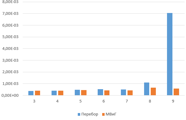
Starting with 9 cities, brute force is noticeably losing. Starting with 13 cities brute force takes more than a minute.
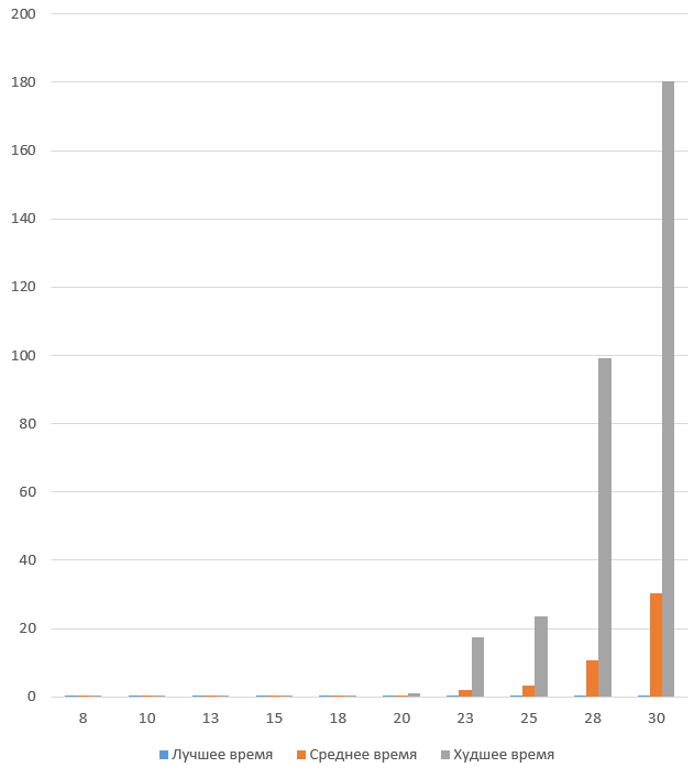
Working hours of the Ministry of Foreign Affairs on a different number of cities
Graphic application
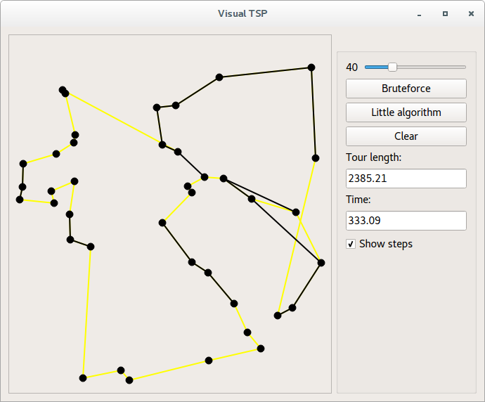
A graphical interface was also made on Qt with the ability to dynamically look at the solution process. Just his working area on the gif in the header of the article. They can compile and touch the prog with their hands.
The yellow color indicates the best path found and its length is in the "Tour length" field.
Black marks the edges that are in the last viewed set.
For dynamic mapping, the problem must be solved either step-by-step, or in a stream parallel to the graphical interface. Since the main solution function is recursive, the second option was chosen, which made it necessary to add a mutex to the decision class, and make the record variable atomic and in some methods take care of thread safety.
Instead of conclusion
I hope this article will help those who want to implement this algorithm or have already implemented and do not understand why it gives the wrong result.
')
Source: https://habr.com/ru/post/332208/
All Articles