Introduction to procedural animation: inverse kinematics

Part 4. Introduction to Gradient Descent

This part is a theoretical introduction to inverse kinematics and contains a software solution based on gradient descent . This article will not be a comprehensive guide on this topic, it is just a general introduction. In the next section, we show the actual implementation of this algorithm in C # in Unity.

The series consists of the following parts (parts 1-3 are presented in the previous post ):

• Part 1. Introduction to procedural animation
• Part 2. Mathematics of direct kinematics
• Part 3. Realization of direct kinematics
• Part 4. Introduction to Gradient Descent
• Part 5. Inverse kinematics for a robotic arm
• Part 6. Inverse kinematics of tentacles
• Part 7. Inverse kinematics of spider legs

Introduction

The previous part of the series (“Realization of direct kinematics”) presents a solution to the problem of direct kinematics . We have a function ForwardKinematics , which defines a point in space, which is currently related to the robot arm.
')
If we have a specific point in space that we want to achieve, then ForwardKinematics can be used to assess the proximity of the manipulator, taking into account the current configuration of the connections. The distance from the target is a function that can be implemented as follows:

 public Vector3 DistanceFromTarget(Vector3 target, float [] angles) { Vector3 point = ForwardKinematics (angles); return Vector3.Distance(point, target); } 

Finding a solution to the problem of inverse kinematics means that we need to minimize the value returned by the DistanceFromTarget function. Minimizing a function is one of the well-known problems, both in programming and in mathematics. The approach we will use is based on a technique called gradient descent ( Wikipedia ). Despite the fact that it is not the most effective, the technique has its advantages: it is not specific to solve a specific problem and there is enough knowledge for it that most programmers have.

Gradient descent

The easiest way to understand the work of gradient descent is to imagine a hilly relief. We are in a random place and want to reach the lowest point. Let's call it a minimum of relief. At each step, the gradient descent tells us to move in a direction that lowers our height. If the geometry of the relief is relatively simple , then this approach will lead us to the very bottom of the valley.

The graph below shows the standard case in which a gradient descent will be successful. In this simplest example, we have a function. It takes one parameter (X axis) and returns the error value (Y axis). We start with a random point on the X axis (blue and green points). Gradient descent should make us move in the direction of the minimum (blue and green arrows).



If we look at the function as a whole, then the direction of motion is obvious. Unfortunately, the gradient descent does not have in advance information about where the minimum is located. The best guess that the algorithm can allow is to move towards a slope, also called a gradient function. If you are on a mountain, release the ball and it will reach the valley. The graph below shows the gradient of the error function at two different points.

Gradient estimate

If you studied mathematical analysis, you probably know that the gradient of a function is directly related to its derivative . However, to calculate the derivative of a function, it is necessary that it satisfy certain mathematical properties, and it is impossible to guarantee the fulfillment of this requirement for any problem in the general case. Moreover, for analytic taking of a derivative, it is necessary that the error function be represented in an analytical form. And we do not always have an analytical view of the function that needs to be minimized.

In all such cases, it is impossible to find the true derivative of the function. The solution is a rough estimate of its value. The graph below shows how it is in one dimension. By discrete sampling of nearby points, the local gradient of the function can be approximately obtained. If the error function is less on the left, then we move to the left, if on the right, then we move to the right.

Maths

Now that we have a general understanding of the graphic work of gradient descent, let's see how to translate it into the language of mathematics. The first step is to calculate the gradient of our error function. at a specific point . We need to find the direction in which the function grows. The gradient of a function is closely related to its derivative. Therefore, it would be nice to start creating our estimate by examining how the derivative is calculated.

Mathematically, the derivative of the function called . Its value is at the point equally , and it shows how fast the function grows. According to her:

• locally grows upwards;
• locally down;
• locally flat.

The idea is to use assessment to calculate the gradient denoted . Mathematically is defined as:



The graph below shows what this means:



In our case, to estimate the derivative, we need to sample the error function at two different points. Short distance between them Is the sampling distance we talked about in the previous section.

Summarize. To calculate the true derivative of the function, you must use the limit. Our gradient is a rough estimate of the derivative created using a fairly small sampling distance:

• Derivative
  
  
  
  
• Approximate gradient
  
  

In the next section, we will see how these two concepts differ with several variables.

Having found the approximate derivative, we need to move in the opposite direction to go down the function. This means that you need to update the parameter. in the following way:



Constant often called learning rate . It determines how fast we will move along the gradient. The greater the value, the faster the solution will be found, but the more likely it is to miss it.

Several variables

The solution we found works in one dimension. This means that we have defined a derivative of the function of the form where Is one number. In this particular case, we can find a fairly accurate approximate value of the derivative of the sample function. at two points: and . The result is a single number indicating an increase or decrease in function. We used this number as a gradient.

The function with one parameter corresponds to a single-joint robot manipulator. If we want to perform a gradient descent for more complex manipulators, then it is necessary to specify the gradient of functions with several variables. For example, if our robotic arm has three joints, the function will be more like . In this case, the gradient is a vector consisting of three numbers showing the local behavior in the three-dimensional space of its parameters.

We can introduce the concept of partial derivatives , which, in essence, are “traditional” derivatives, calculated for each of the variables:







They represent three different scalar numbers, each of which shows how the function grows in a certain direction (or along the axis). To calculate the total gradient, we approximate each partial derivative with a corresponding gradient using sufficiently small sample distances. , and :







For our gradient descent, we will use a vector containing all three results as the gradient:

Part 5. Inverse kinematics for a robotic arm

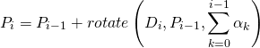
After a long journey into mathematics of direct kinematics and geometric analysis of gradient descent, we are finally ready to demonstrate the working implementation of the problem of inverse kinematics. In this section, we will show how it can be applied to a robot manipulator, similar to the one shown below.

Introduction

The previous part outlines the mathematical foundations of a technique called gradient descent . We have a function receiving parameter each joint of the robot manipulator. This parameter is the current joint angle. For a given articulation configuration function returns one value indicating how far the final link of the manipulator robot is from the target point . Our task is to find the values. minimizing .

To do this, we first calculate the gradient of the function at the current . Gradient is a vector showing the direction of the fastest climb. Simply put, this is an arrow indicating the direction in which the function grows. Each element of the gradient is an approximate value of the partial derivative. .

For example, if a robotic arm has three joints, then we will have a function that takes three parameters: , and . Then our gradient is set as:



Where:







but , and - sufficiently small values.

We got an approximate gradient . If we want to minimize then you need to move in the opposite direction. This means an update. , and in the following way:







Where - this is the learning rate , a positive parameter that controls the speed of removal from the rising gradient.

Implementation

Now we have all the knowledge necessary to implement a simple gradient descent in C #. Let's start with a function that calculates the approximate value of the partial gradient of the i -th articulation. As mentioned above, for this we need to create a function sample. (which is our error function DistanceFromTarget , described in “Introducing Gradient Descent”) at two points:

 public float PartialGradient (Vector3 target, float[] angles, int i) { //  , //     float angle = angles[i]; // : [F(x+SamplingDistance) - F(x)] / h float f_x = DistanceFromTarget(target, angles); angles[i] += SamplingDistance; float f_x_plus_d = DistanceFromTarget(target, angles); float gradient = (f_x_plus_d - f_x) / SamplingDistance; //  angles[i] = angle; return gradient; } 

When this function is called, it returns a single number that determines how the distance from the target changes as a function of the rotation of the joint.

We need to cycle through all the joints, calculating their effect on the gradient.

 public void InverseKinematics (Vector3 target, float [] angles) { for (int i = 0; i < Joints.Length; i ++) { //   //  : Solution -= LearningRate * Gradient float gradient = PartialGradient(target, angles, i); angles[i] -= LearningRate * gradient; } } 

Repeated calls to InverseKinematics move the robotic arm closer to the target point.

Premature termination

One of the main problems of inverse kinematics implemented by this naive approach is the low probability of the final convergence of the gradient. Depending on the values ​​chosen for LearningRate and SamplingDistance very possible that the manipulator will “swing” alongside the true solution.



This is because we update the corners too often, and this leads to a “hop” over the true point. The correct solution to this problem is the use of adaptive learning rate, which varies depending on the proximity to the solution. A cheaper alternative is to stop the optimization algorithm if we are closer than a certain threshold value:

 public void InverseKinematics (Vector3 target, float [] angles) { if (DistanceFromTarget(target, angles) < DistanceThreshold) return; for (int i = Joints.Length -1; i >= 0; i --) { //   //  : Solution -= LearningRate * Gradient float gradient = PartialGradient(target, angles, i); angles[i] -= LearningRate * gradient; //   if (DistanceFromTarget(target, angles) < DistanceThreshold) return; } } 

If we repeat this check after each rotation of the articulation, we will perform the minimum number of movements required.

To further optimize the motion of the manipulator, we can apply a gradient descent in the reverse order. If we start at the end link and not at the bottom, this will allow us to make shorter movements. In general, these small tricks allow you to get closer to a more natural solution.

Restrictions

One of the characteristics of real joints is that they usually have a limited range of possible angles of rotation. Not all joints can rotate 360 ​​degrees around its axis. So far we have not imposed any restrictions on our optimization algorithm. This means that we are likely to get this behavior:



The solution is pretty obvious. We will add minimum and maximum angles to the RobotJoint class:

 using UnityEngine; public class RobotJoint : MonoBehaviour { public Vector3 Axis; public Vector3 StartOffset; public float MinAngle; public float MaxAngle; void Awake () { StartOffset = transform.localPosition; } } 

then you need to make sure that we limit the corners to the desired range:

 public void InverseKinematics (Vector3 target, float [] angles) { if (DistanceFromTarget(target, angles) < DistanceThreshold) return; for (int i = Joints.Length -1; i >= 0; i --) { //   //  : Solution -= LearningRate * Gradient float gradient = PartialGradient(target, angles, i); angles[i] -= LearningRate * gradient; //  angles[i] = Mathf.Clamp(angles[i], Joints[i].MinAngle, Joints[i].MaxAngle); //   if (DistanceFromTarget(target, angles) < DistanceThreshold) return; } } 

Problems

Even with limited angles and premature termination, the algorithm we used is very simple. Too simple. Many problems can arise with this solution, and most of them are associated with a gradient descent. As it is written in “Introducing Gradient Descent,” the algorithm can get stuck in local minima . They are suboptimal solutions : unnatural or undesirable ways of achieving the goal.

Look at the animation:


The arm of the manipulator went too far, and when it returned to its original position, it turned over.The best way to avoid this is to use the comfort function . If we have reached the required point, then we need to try to change the orientation of the manipulator to a more comfortable, natural position. It should be noted that this is not always possible. Changing the orientation of the manipulator can cause the algorithm to increase the distance to the target, which may contradict its parameters.

Part 6. Inverse kinematics of tentacles

Introduction

In the previous section, we explored the use of gradient descent to implement the inverse kinematics of a robotic arm. The movement performed by mechanisms is quite simple, because they do not have the complexity of real human body parts. Each joint of the robotic arm is controlled by the engine. In the human body, each muscle is de facto an independent motor that can stretch and contract.

Some creatures have body parts that have several degrees of freedom. An example is the trunk of an elephant and the tentacle of an octopus. Modeling such body parts is a particularly difficult task, because the above traditional techniques cannot create realistic results.

We will start with an example from the previous part and gradually come to a behavior that will be quite realistic for our purposes.

Tentacle rigging

In the robot manipulator we created, each part moved independently of the others. Tentacles, unlike a robot, can be bent. This is a necessary feature that cannot be ignored if we want to focus on realism. Our tentacle must be able to bend.

The Unity component that allows this feature to be implemented is called Skinned Mesh Renderer :


Unfortunately, Unity does not provide the ability to create a skinning mesh renderer in the editor. A 3D model editor is required, for example, Blender . The image below shows the tentacle model that we will use in this part. Inside you can see several bones connected to each other. These are objects that allow us to bend the model.


In this tutorial, we will not explore adding bones to models, also called rigging . A good introduction to the subject can be found in the Blender 3D article : Noob to Pro / Bones .

Bones and joints

The next stage of realization of the inverse tentacle kinematics is the attachment of a script to each bone RobotJoint. Because of this, we give our inverse kinematics algorithm the opportunity to bend the tentacle.

In a normal octopus, each joint can rotate freely in all three axes. Unfortunately, the code written for the robot manipulator allows rotation of the joints along one axis only. If we try to change this, we will add a new level of complexity to our code. Instead, we can cyclically change the axis of the joints so that the joint 0 turns in X, the joint 1 in Y, the joint 2 in Z, and so on. This can lead to unnatural behavior, but such a problem you may never have if the bones are small enough.

In the downloadable Unity project sold with this tutorial, the script SetRobotJointWeightsautomatically initializes the parameters of all tentacle junctions. You can do it manually to have more precise control over the movement of each bone.

Comfort function

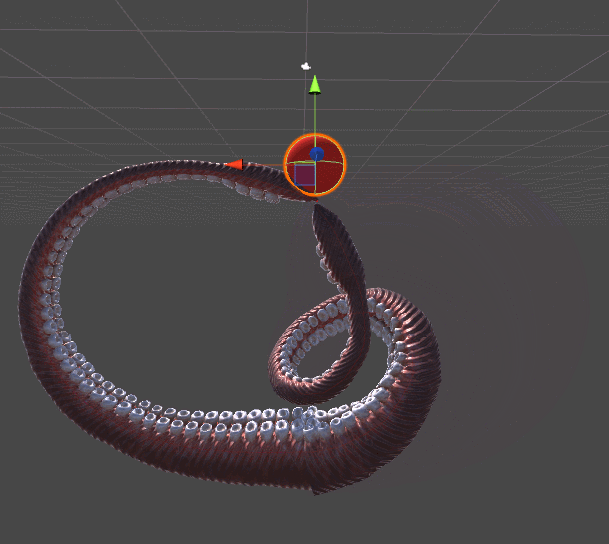
The animation below shows two tentacles. The tentacle on the left stretches to the red sphere using an algorithm from Inverse Kinematics for a Robotic Arm. The right tentacle adds a whole new level of realism, twisting spirally, in a more organic style. This example should be enough to understand why the tentacles need their own tutorial.


Gradient descent is used for both tentacles. The difference lies in the error function , which they seek to minimize. The mechanical tentacle on the left simply seeks to reach the ball, it does not care about all the other parameters. As soon as the final link touches the ball, the approach is considered complete and the tentacle just stops moving.

The tentacle on the right minimizes another function. The function DistanceFromTargetused for the manipulator is replaced with a new, more complex function. We can make this new feature ErrorFunctiontake into account other parameters that are important to us. Tentacles shown in this tutorial minimize three different functions:

• Distance to target : ready
  
  
• : , . , . , , . , . . Unity — Quaternion.Angle :
  
  

   float rotationPenalty = Mathf.Abs ( Quaternion.Angle(EndEffector.rotation, Destination.rotation) / 180f ); 

  
  . .
  
  
• Torsion : keep parts of the body unnaturally uncomfortable. This parameter “penalizes” curvilinear motions, causing inverse kinematics to perform a more linear, simple turn. To calculate the penalty for torsion, we first need to determine what “torsion” is in this context. It is easiest to define it as the average angle for all joints. Such a penalty tends to keep the tentacle relaxed, and “punishes” solutions that require a large number of bends.
  
  

   float torsionPenalty = 0; for (int i = 0; i < solution.Length; i++) torsionPenalty += Mathf.Abs(solution[i]); torsionPenalty /= solution.Length; 

These three limitations lead to a more realistic tentacle movement. A more complex version can provide fluctuations, even when the conditions satisfy all other restrictions.

Enhancements

Practically there are no restrictions for making improvements to our model. Improving the realism of the tentacles will definitely help slowdown function. Tentacles should move slower when approaching the goal.

In addition, the tentacles should not intersect each other. To avoid this, use colliders for each joint. However, this can lead to freakish behavior. In our code, collisions are ignored and it can come closer to a solution in which self-intersections occur. The solution is to change the fitness function so that solutions with self-intersection have high penalties.

[A ready-made Unity project with scripts and 3D models can be purchased for $ 10 on the Patreon page of the author of the original article.]

, , . :