Autoencoders in Keras, Part 6: VAE + GAN

Content

Part 1: Introduction
Part 2: Manifold learning and latent variables
Part 3: Variational autoencoders ( VAE )
Part 4: Conditional VAE
Part 5: GAN (Generative Adversarial Networks) and tensorflow
Part 6: VAE + GAN

In the previous part, we created a CVAE autoencoder, whose decoder is able to generate a digit of a given label, we also tried to create pictures of numbers of other labels in the style of a given picture. It turned out pretty good, but the numbers were generated blurry.

In the last part, we studied how the GANs work, getting quite clear images of numbers, but the possibility of coding and transferring the style was lost.

In this part we will try to take the best from both approaches by combining variational autoencoders ( VAE ) and generative competing networks ( GAN ).
')
The approach, which will be described later, is based on the article [Autoencoding beyond pixels using a learned similarity metric, Larsen et al, 2016] .

Illustration of [1]

We will understand in more detail why the recovered images are blurry.

In the part about VAE , the process of image generation was considered.

from latent variables

.
Since the dimension of hidden variables

significantly lower than the dimension of objects

(in the part about VAE, these dimensions were 2 and 784), and there is always some randomness, then the same

may correspond to multidimensional distribution

, i.e

. This distribution can be represented as:

$P (X | Z) = f (Z) + \ epsilon,$

Where

some average most likely object for a given

, but $\ epsilon$ - the noise of a complex nature.

When we train autoencoders, we compare the input from the sample X_s

and autoencoder exit $\ tilde X_s$ using some error functional

$L (X_s, \ tilde X_s), \\ \ tilde X_s = f_d (Z; \ theta_d), \\ Z \ sim Q (Z | X_s; \ theta_e),$

Where $Q, \ f_d$ - encoder and decoder.

Asking

we define noise $\ epsilon_L$ which bring real noise $\ epsilon$ .
Minimizing

, we teach autoencoder to adapt to noise $\ epsilon_L$ , removing it, that is, to find the average value in a given metric (in the second part it was shown visually on a simple artificial example).

If the noise $\ epsilon_L$ which we define as functional

does not match the actual noise $\ epsilon$ then $f_d (Z; \ theta_2)$ prove to be greatly biased from real f (z)

(example: if the real noise in the regression is laplassovsky, and the difference of squares is minimized, then the predicted value will be shifted towards emissions).

Returning to the pictures: let's see how the pixel metric is connected, which defines the loss in the previous parts, and the metric used by the person. An example and illustration from [2] :

In the picture above:
(a) - the original image of the digit,
(b) - obtained from (a) by cutting a piece,
(c) is the digit (a) shifted half a pixel to the right.

In terms of per-pixel metric, (a) is much closer to (b) than to (c); although from the point of view of human perception (b) is not even a figure, but the difference between (a) and (b) is almost imperceptible.

Autoencoders with a pixel-by-pixel metric thus blurred the image, reflecting the fact that within the limits of close

the position of the figures slightly walks in the picture,
figures are drawn slightly differently (although pixel-by-pixel can be far away).

According to the metrics of human perception, the fact that the figure has blurred already makes it be very different from the original. Thus, if we know the person’s metric or close to it and optimize in it, the numbers will not be eroded, and the importance of the figure being full, not like from the picture (b), will increase dramatically.

You can try to manually invent a metric that will be closer to the human. But using the GAN approach, it is possible to train the neural network to look for a good metric itself.

About GAN'y written in the last part.

Connecting VAE and GAN

The GAN generator performs a function similar to the decoder in VAE : both samples are from a prior distribution P (Z)

and translate it into P_g (X)

. However, they have different roles: the decoder restores the object encoded by the encoder, while learning based on some comparison metric; the generator, on the other hand, generates a random object that is not compared with anything, so long as the discriminator cannot distinguish which of the distributions

he belongs

The idea is to add a third network to the VAE - the discriminator and feed the input and the restored object and the original to it, and train the discriminator to determine which one is which.

Illustration of [1]

Of course, we can no longer use the same comparison metric from VAE , because, while studying in it, the decoder generates images that are easily distinguishable from the original. Do not use the metric at all - either, since we would like the recreated $\ tilde X$ looked like the original and not just some random of P (X)

as in pure gan .

Let us think, however, about this: the discriminator, learning to distinguish between a real object and a generated one, will isolate some characteristic features of one and the other. These features of the object will be encoded in the layers of the discriminator, and based on their combination, it will already give the probability of the object to be real. For example, if the image is blurred, then some kind of neuron in the discriminator will activate more strongly than if it is clear. Moreover, the deeper the layer, the more abstract characteristics of the input object are encoded in it.

Since each discriminator layer is a code-description of an object and at the same time encodes features that allow the discriminator to distinguish generated objects from real ones, it is possible to replace some simple metric (for example, pixel-by-pixel) with a metric over neuronal activations in one of the layers:

$L (X_s, \ tilde X_s) \ longrightarrow L_d (d_l (X_s), d_l (\ tilde X_s)) \\ \ tilde X_s = f_d (Z; \ theta_d), \\ Z \ sim Q (X_s; \ theta_e) ,$

Where

- activation on

th layer of the discriminator, and $Q, \ f_d$ - encoder and decoder.

At the same time, it is hoped that the new metric L_d

will be better.

Below is a diagram of the work of the resulting VAE + GAN network, proposed by the authors [1] .

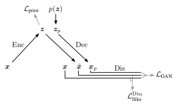
Illustration of [1]

Here:

- input object from ,
- sampled of ,
- object generated by decoder from ,
$\ tilde X$ - object recovered from ,
$\ mathcal L_ {prior} = KL \ left [Q (Z | X) || P (Z) \ right]$ - loss forcing the encoder to translate in the right for us (just like in part 3 about VAE ),
$\ mathcal L_ {llike} ^ {Dis_l} = L_d (d_l (X), d_l (\ tilde X))$ - metric between activations layer of discriminator on real and restored $\ tilde X = f_d (Q (X))$ ,
$\ mathcal L_ {GAN} = \ log (D (X)) + \ log (1 - D (f_d (Z))) + \ log (1 - D (f_d (Q (X))))$ - cross-entropy between the real distribution of labels of real / generated objects, and the probability distribution predicted by the discriminator.

As with the GAN , we cannot train all 3 parts of the network at the same time. The discriminator should be trained separately, in particular, it is not necessary that the discriminator try to reduce $\ mathcal L_ {llike} ^ {Dis_l}$ , since it will collapse the difference of activations in 0. Therefore, the training of all networks should be limited only to their relevant losses.

The scheme proposed by the authors:

$\ theta_ {Enc} = \ theta_ {Enc} - \ Delta _ {\ theta_ {Enc}} (\ mathcal L_ {prior} + \ mathcal L ^ {Dis_l} _ {llike}), \\ \ theta_ {Dec} = \ theta_ {Dec} - \ Delta _ {\ theta_ {Dec}} (\ gamma \ mathcal L ^ {Dis_l} _ {llike} - \ mathcal L_ {GAN}), \\ \ theta_ {Dis} = \ theta_ {Dis } - \ Delta _ {\ theta_ {Dis}} (\ mathcal L_ {GAN})$

Above it can be seen on which Loss what networks study. Particular attention should be paid to the decoder: on the one hand, it tries to reduce the distance between the input and the output in the metric of the lth discriminator layer ( $\ mathcal L ^ {Dis_l} _ {llike}$ ), on the other hand, trying to trick the discriminator (by increasing $\ mathcal L_ {GAN}$ ). In the article, the authors argue that by changing the coefficient $\ gamma$ , you can influence what is more important for the network: content ( $\ mathcal L ^ {Dis_l} _ {llike}$ ) or style ( $\ mathcal L_ {GAN}$ ). I can not, however, say that I have observed this effect.

Code

The code largely repeats what was in the previous parts about pure VAE and GAN .

Again, we will immediately write the conditional model.

from IPython.display import clear_output import numpy as np import matplotlib.pyplot as plt %matplotlib inline import seaborn as sns from keras.layers import Dropout, BatchNormalization, Reshape, Flatten, RepeatVector from keras.layers import Lambda, Dense, Input, Conv2D, MaxPool2D, UpSampling2D, concatenate from keras.layers.advanced_activations import LeakyReLU from keras.layers import Activation from keras.models import Model, load_model #    keras from keras import backend as K import tensorflow as tf sess = tf.Session() K.set_session(sess) #   from keras.datasets import mnist from keras.utils import to_categorical (x_train, y_train), (x_test, y_test) = mnist.load_data() x_train = x_train.astype('float32') / 255. x_test = x_test .astype('float32') / 255. x_train = np.reshape(x_train, (len(x_train), 28, 28, 1)) x_test = np.reshape(x_test, (len(x_test), 28, 28, 1)) y_train_cat = to_categorical(y_train).astype(np.float32) y_test_cat = to_categorical(y_test).astype(np.float32) #   batch_size = 64 batch_shape = (batch_size, 28, 28, 1) latent_dim = 8 num_classes = 10 dropout_rate = 0.3 gamma = 1 #   #      def gen_batch(x, y): n_batches = x.shape[0] // batch_size while(True): idxs = np.random.permutation(y.shape[0]) x = x[idxs] y = y[idxs] for i in range(n_batches): yield x[batch_size*i: batch_size*(i+1)], y[batch_size*i: batch_size*(i+1)] train_batches_it = gen_batch(x_train, y_train_cat) test_batches_it = gen_batch(x_test, y_test_cat) #   x_ = tf.placeholder(tf.float32, shape=(None, 28, 28, 1), name='image') y_ = tf.placeholder(tf.float32, shape=(None, 10), name='labels') z_ = tf.placeholder(tf.float32, shape=(None, latent_dim), name='z') img = Input(tensor=x_) lbl = Input(tensor=y_) z = Input(tensor=z_)

The description of models from GAN differs almost only in the added encoder.

 def add_units_to_conv2d(conv2, units): dim1 = int(conv2.shape[1]) dim2 = int(conv2.shape[2]) dimc = int(units.shape[1]) repeat_n = dim1*dim2 units_repeat = RepeatVector(repeat_n)(lbl) units_repeat = Reshape((dim1, dim2, dimc))(units_repeat) return concatenate([conv2, units_repeat]) #   ,  -        (,  - ,  P  P_g   ) def apply_bn_relu_and_dropout(x, bn=False, relu=True, dropout=True): if bn: x = BatchNormalization(momentum=0.99, scale=False)(x) if relu: x = LeakyReLU()(x) if dropout: x = Dropout(dropout_rate)(x) return x with tf.variable_scope('encoder'): x = Conv2D(32, kernel_size=(3, 3), strides=(2, 2), padding='same')(img) x = apply_bn_relu_and_dropout(x) x = MaxPool2D((2, 2), padding='same')(x) x = Conv2D(64, kernel_size=(3, 3), padding='same')(x) x = apply_bn_relu_and_dropout(x) x = Flatten()(x) x = concatenate([x, lbl]) h = Dense(64)(x) h = apply_bn_relu_and_dropout(h) z_mean = Dense(latent_dim)(h) z_log_var = Dense(latent_dim)(h) def sampling(args): z_mean, z_log_var = args epsilon = K.random_normal(shape=(batch_size, latent_dim), mean=0., stddev=1.0) return z_mean + K.exp(K.clip(z_log_var/2, -2, 2)) * epsilon l = Lambda(sampling, output_shape=(latent_dim,))([z_mean, z_log_var]) encoder = Model([img, lbl], [z_mean, z_log_var, l], name='Encoder') with tf.variable_scope('decoder'): x = concatenate([z, lbl]) x = Dense(7*7*128)(x) x = apply_bn_relu_and_dropout(x) x = Reshape((7, 7, 128))(x) x = UpSampling2D(size=(2, 2))(x) x = Conv2D(64, kernel_size=(5, 5), padding='same')(x) x = apply_bn_relu_and_dropout(x) x = Conv2D(32, kernel_size=(3, 3), padding='same')(x) x = UpSampling2D(size=(2, 2))(x) x = apply_bn_relu_and_dropout(x) decoded = Conv2D(1, kernel_size=(5, 5), activation='sigmoid', padding='same')(x) decoder = Model([z, lbl], decoded, name='Decoder') with tf.variable_scope('discrim'): x = Conv2D(128, kernel_size=(7, 7), strides=(2, 2), padding='same')(img) x = MaxPool2D((2, 2), padding='same')(x) x = apply_bn_relu_and_dropout(x) x = add_units_to_conv2d(x, lbl) x = Conv2D(64, kernel_size=(3, 3), padding='same')(x) x = MaxPool2D((2, 2), padding='same')(x) x = apply_bn_relu_and_dropout(x) # l-      l = Conv2D(16, kernel_size=(3, 3), padding='same')(x) x = apply_bn_relu_and_dropout(x) h = Flatten()(x) d = Dense(1, activation='sigmoid')(h) discrim = Model([img, lbl], [d, l], name='Discriminator')

Building a graph of calculations based on models:

 z_mean, z_log_var, encoded_img = encoder([img, lbl]) decoded_img = decoder([encoded_img, lbl]) decoded_z = decoder([z, lbl]) discr_img, discr_l_img = discrim([img, lbl]) discr_dec_img, discr_l_dec_img = discrim([decoded_img, lbl]) discr_dec_z, discr_l_dec_z = discrim([decoded_z, lbl]) cvae_model = Model([img, lbl], decoder([encoded_img, lbl]), name='cvae') cvae = cvae_model([img, lbl])

Loss Definition:

Interestingly, the result was slightly better if the cross-entropy rather than MSE was taken as the metric for layer activations.

 #   L_prior = -0.5*tf.reduce_sum(1. + tf.clip_by_value(z_log_var, -2, 2) - tf.square(z_mean) - tf.exp(tf.clip_by_value(z_log_var, -2, 2)))/28/28 log_dis_img = tf.log(discr_img + 1e-10) log_dis_dec_z = tf.log(1. - discr_dec_z + 1e-10) log_dis_dec_img = tf.log(1. - discr_dec_img + 1e-10) L_GAN = -1/4*tf.reduce_sum(log_dis_img + 2*log_dis_dec_z + log_dis_dec_img)/28/28 # L_dis_llike = tf.reduce_sum(tf.square(discr_l_img - discr_l_dec_img))/28/28 L_dis_llike = tf.reduce_sum(tf.nn.sigmoid_cross_entropy_with_logits(labels=tf.sigmoid(discr_l_img), logits=discr_l_dec_img))/28/28 #  , ,  L_enc = L_dis_llike + L_prior L_dec = gamma * L_dis_llike - L_GAN L_dis = L_GAN #    optimizer_enc = tf.train.RMSPropOptimizer(0.001) optimizer_dec = tf.train.RMSPropOptimizer(0.0003) optimizer_dis = tf.train.RMSPropOptimizer(0.001) encoder_vars = tf.get_collection(tf.GraphKeys.TRAINABLE_VARIABLES, "encoder") decoder_vars = tf.get_collection(tf.GraphKeys.TRAINABLE_VARIABLES, "decoder") discrim_vars = tf.get_collection(tf.GraphKeys.TRAINABLE_VARIABLES, "discrim") step_enc = optimizer_enc.minimize(L_enc, var_list=encoder_vars) step_dec = optimizer_dec.minimize(L_dec, var_list=decoder_vars) step_dis = optimizer_dis.minimize(L_dis, var_list=discrim_vars) def step(image, label, zp): l_prior, dec_image, l_dis_llike, l_gan, _, _ = sess.run([L_prior, decoded_z, L_dis_llike, L_GAN, step_enc, step_dec], feed_dict={z:zp, img:image, lbl:label, K.learning_phase():1}) return l_prior, dec_image, l_dis_llike, l_gan def step_d(image, label, zp): l_gan, _ = sess.run([L_GAN, step_dis], feed_dict={z:zp, img:image, lbl:label, K.learning_phase():1}) return l_gan

Functions of drawing pictures after and during the training:

Code

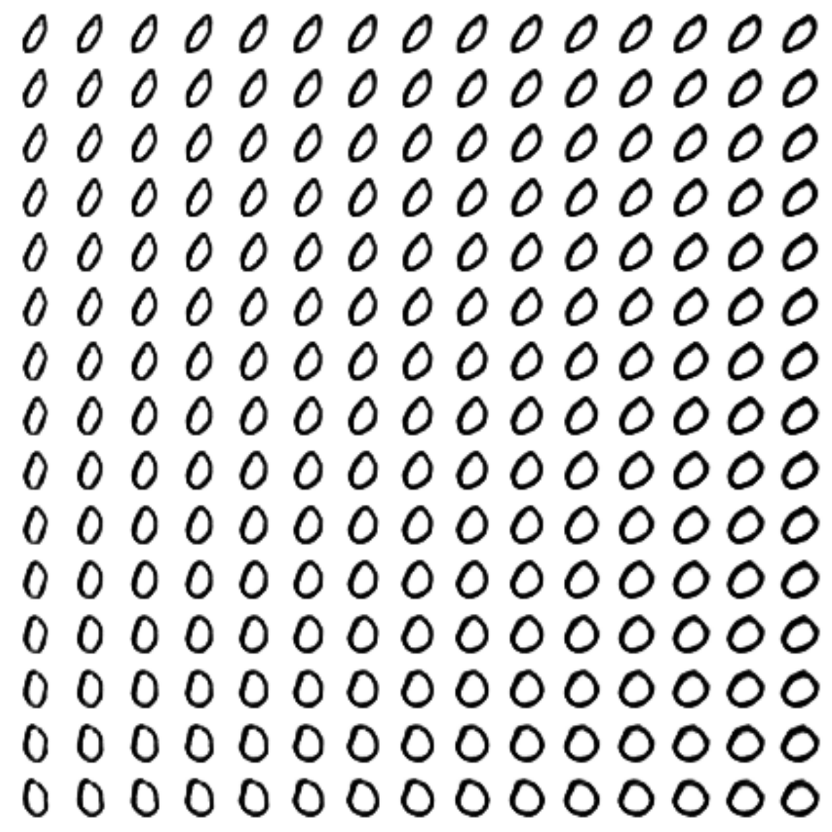
 digit_size = 28 def plot_digits(*args, invert_colors=False): args = [x.squeeze() for x in args] n = min([x.shape[0] for x in args]) figure = np.zeros((digit_size * len(args), digit_size * n)) for i in range(n): for j in range(len(args)): figure[j * digit_size: (j + 1) * digit_size, i * digit_size: (i + 1) * digit_size] = args[j][i].squeeze() if invert_colors: figure = 1-figure plt.figure(figsize=(2*n, 2*len(args))) plt.imshow(figure, cmap='Greys_r') plt.grid(False) ax = plt.gca() ax.get_xaxis().set_visible(False) ax.get_yaxis().set_visible(False) plt.show() # ,     ,    figs = [[] for x in range(num_classes)] periods = [] save_periods = list(range(100)) + list(range(100, 1000, 10)) n = 15 #   15x15  from scipy.stats import norm #     N(0, I),   ,          grid_x = norm.ppf(np.linspace(0.05, 0.95, n)) grid_y = norm.ppf(np.linspace(0.05, 0.95, n)) grid_y = norm.ppf(np.linspace(0.05, 0.95, n)) def draw_manifold(label, show=True): #     figure = np.zeros((digit_size * n, digit_size * n)) input_lbl = np.zeros((1, 10)) input_lbl[0, label] = 1 for i, yi in enumerate(grid_x): for j, xi in enumerate(grid_y): z_sample = np.zeros((1, latent_dim)) z_sample[:, :2] = np.array([[xi, yi]]) x_decoded = sess.run(decoded_z, feed_dict={z:z_sample, lbl:input_lbl, K.learning_phase():0}) digit = x_decoded[0].squeeze() figure[i * digit_size: (i + 1) * digit_size, j * digit_size: (j + 1) * digit_size] = digit if show: #  plt.figure(figsize=(15, 15)) plt.imshow(figure, cmap='Greys') plt.grid(False) ax = plt.gca() ax.get_xaxis().set_visible(False) ax.get_yaxis().set_visible(False) plt.show() return figure #   z def draw_z_distr(z_predicted): im = plt.scatter(z_predicted[:, 0], z_predicted[:, 1]) im.axes.set_xlim(-5, 5) im.axes.set_ylim(-5, 5) plt.show() def on_n_period(period): n_compare = 10 clear_output() #   output #      b = next(test_batches_it) decoded = sess.run(cvae, feed_dict={img:b[0], lbl:b[1], K.learning_phase():0}) plot_digits(b[0][:n_compare], decoded[:n_compare]) #     y draw_lbl = np.random.randint(0, num_classes) print(draw_lbl) for label in range(num_classes): figs[label].append(draw_manifold(label, show=label==draw_lbl)) xs = x_test[y_test == draw_lbl] ys = y_test_cat[y_test == draw_lbl] z_predicted = sess.run(z_mean, feed_dict={img:xs, lbl:ys, K.learning_phase():0}) draw_z_distr(z_predicted) periods.append(period)

Learning process:

 sess.run(tf.global_variables_initializer()) nb_step = 3 #      batches_per_period = 3 for i in range(48000): print('.', end='') #    for j in range(nb_step): b0, b1 = next(train_batches_it) zp = np.random.randn(batch_size, latent_dim) l_g = step_d(b0, b1, zp) if l_g < 1.0: break #      for j in range(nb_step): l_p, zx, l_d, l_g = step(b0, b1, zp) if l_g > 0.4: break b0, b1 = next(train_batches_it) zp = np.random.randn(batch_size, latent_dim) #    if not i % batches_per_period: period = i // batches_per_period if period in save_periods: on_n_period(period) print(i, l_p, l_d, l_g)

Gif drawing function:

Code

 from matplotlib.animation import FuncAnimation from matplotlib import cm import matplotlib def make_2d_figs_gif(figs, periods, c, fname, fig, batches_per_period): norm = matplotlib.colors.Normalize(vmin=0, vmax=1, clip=False) im = plt.imshow(np.zeros((28,28)), cmap='Greys', norm=norm) plt.grid(None) plt.title("Label: {}\nBatch: {}".format(c, 0)) def update(i): im.set_array(figs[i]) im.axes.set_title("Label: {}\nBatch: {}".format(c, periods[i]*batches_per_period)) im.axes.get_xaxis().set_visible(False) im.axes.get_yaxis().set_visible(False) return im anim = FuncAnimation(fig, update, frames=range(len(figs)), interval=100) anim.save(fname, dpi=80, writer='ffmpeg') for label in range(num_classes): make_2d_figs_gif(figs[label], periods, label, "./figs6/manifold_{}.mp4".format(label), plt.figure(figsize=(10,10)), batches_per_period)

Since we again have a model based on autoencoder, we can apply the style transfer:

Code

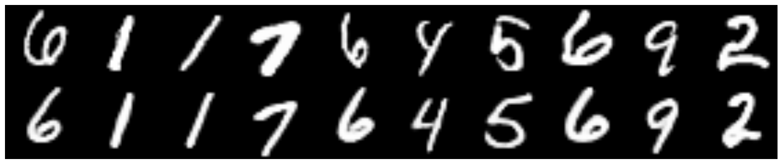
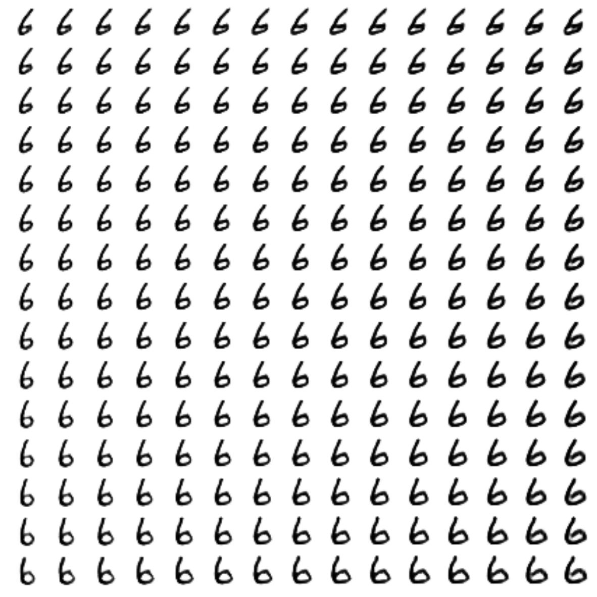
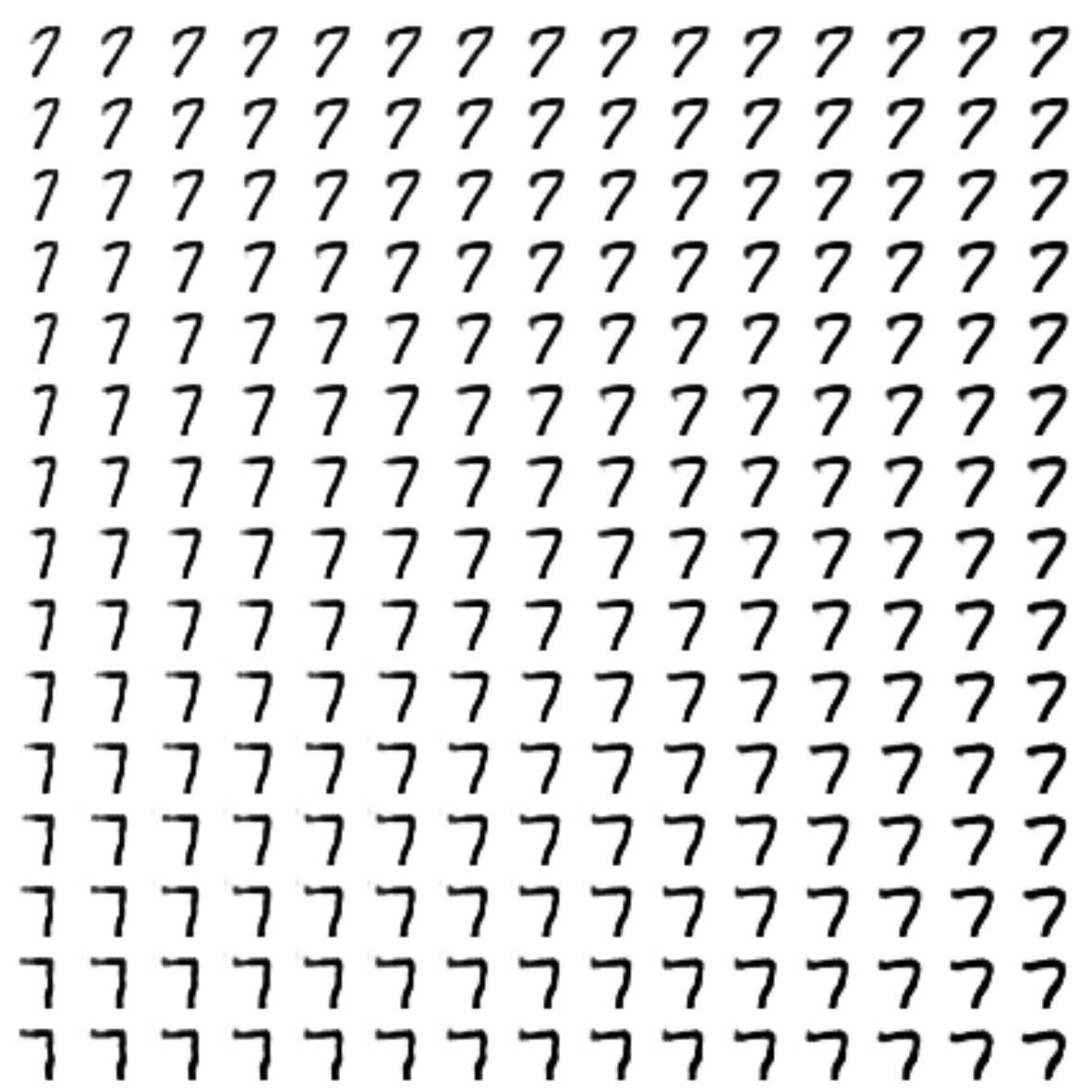
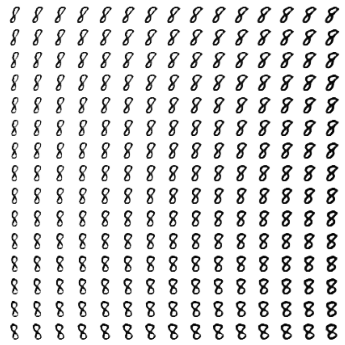
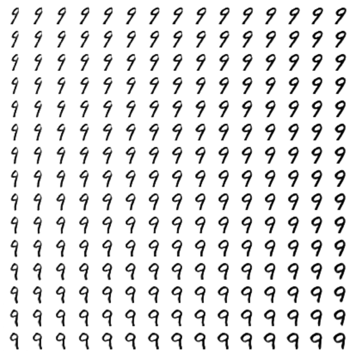
 #   def style_transfer(X, lbl_in, lbl_out): rows = X.shape[0] if isinstance(lbl_in, int): label = lbl_in lbl_in = np.zeros((rows, 10)) lbl_in[:, label] = 1 if isinstance(lbl_out, int): label = lbl_out lbl_out = np.zeros((rows, 10)) lbl_out[:, label] = 1 #     zp = sess.run(z_mean, feed_dict={img:X, lbl:lbl_in, K.learning_phase():0}) #    ,   created = sess.run(decoded_z, feed_dict={z:zp, lbl:lbl_out, K.learning_phase():0}) return created #    def draw_random_style_transfer(label): n = 10 generated = [] idxs = np.random.permutation(y_test.shape[0]) x_test_permut = x_test[idxs] y_test_permut = y_test[idxs] prot = x_test_permut[y_test_permut == label][:batch_size] for i in range(num_classes): generated.append(style_transfer(prot, label, i)[:n]) generated[label] = prot plot_digits(*generated, invert_colors=True) draw_random_style_transfer(7)

results

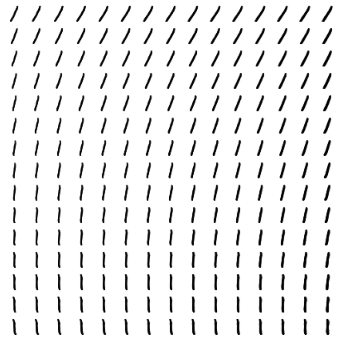
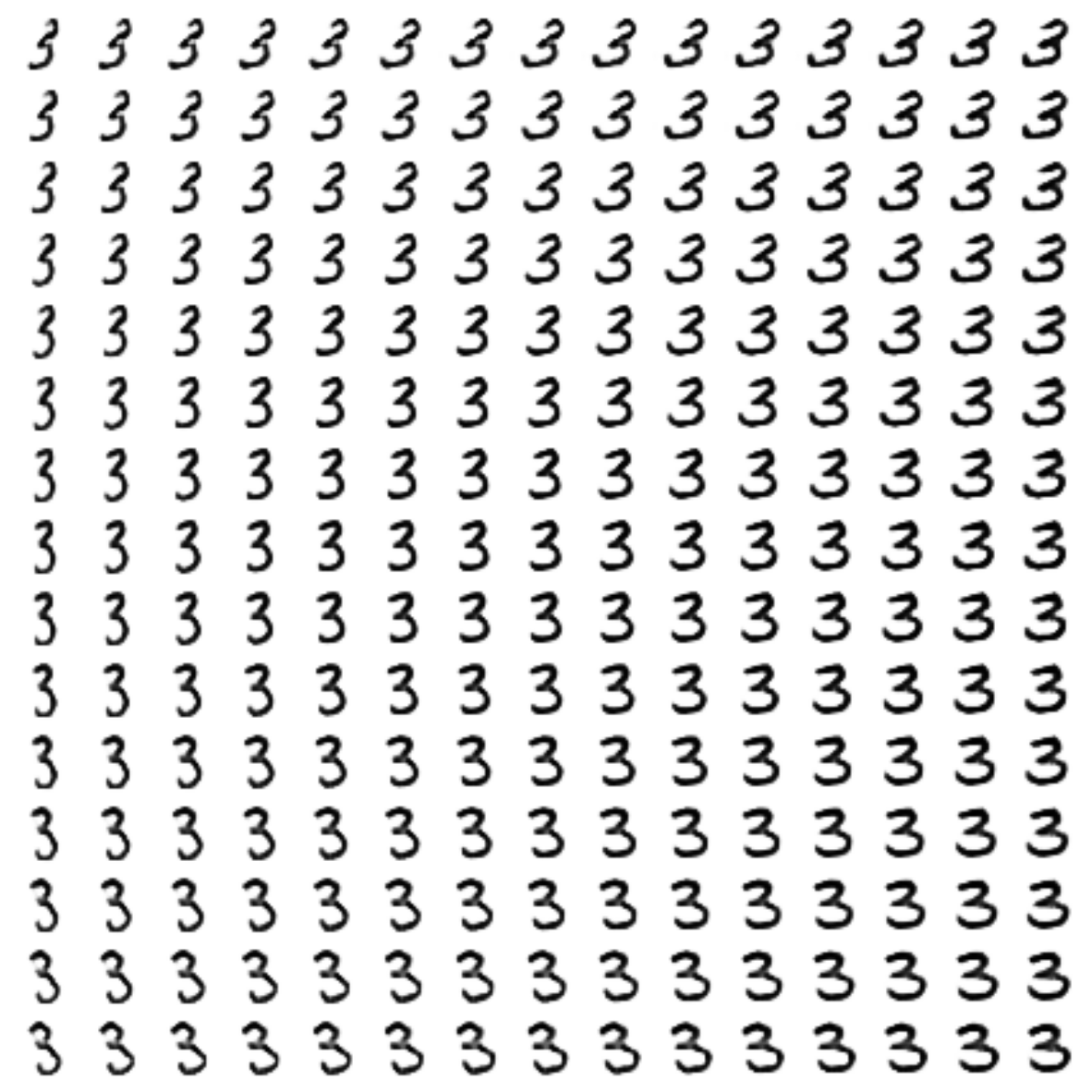
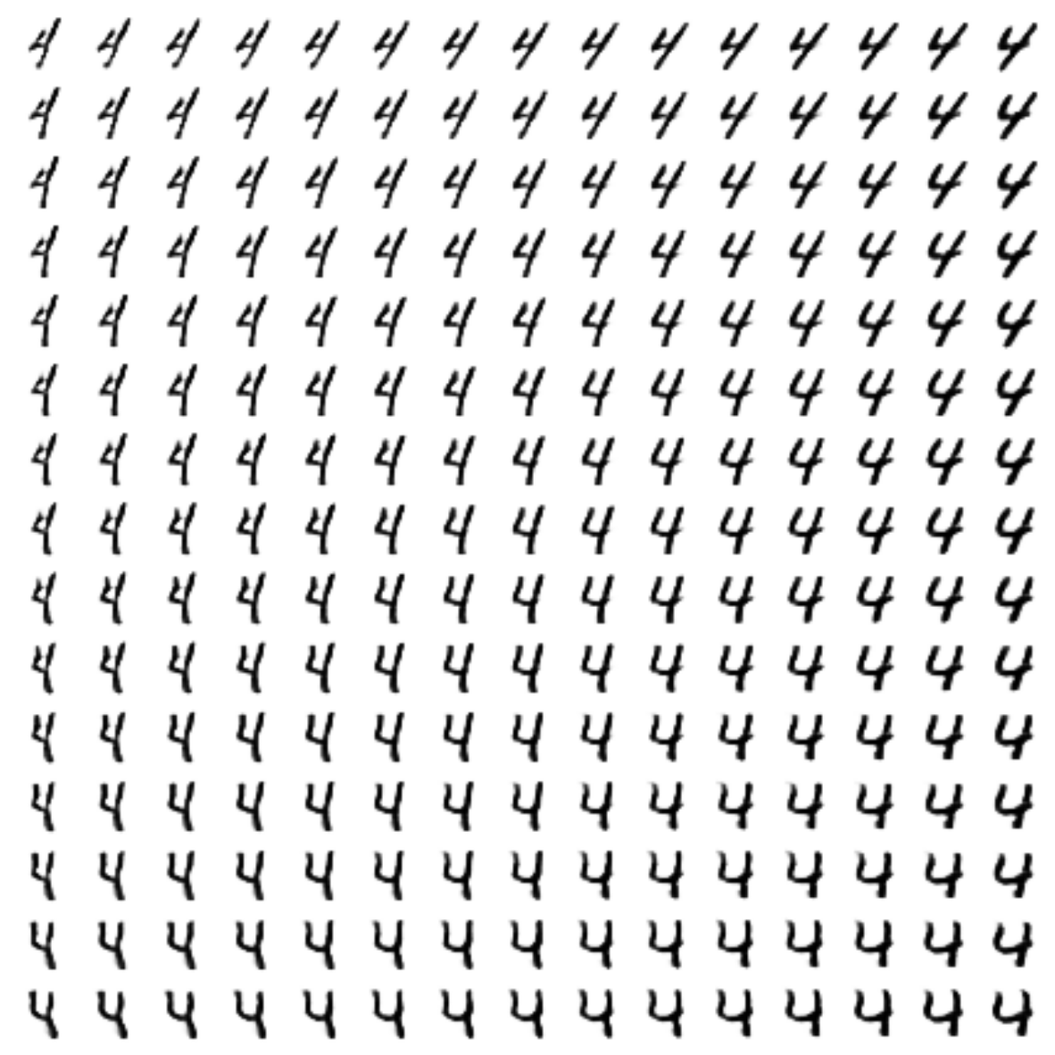
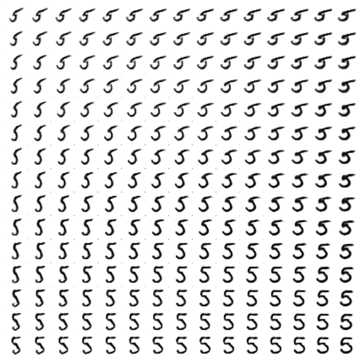
Comparison with a simple CVAE

Top of the original figures, recovered from the bottom.

CVAE , hidden dimension - 2

CVAE + GAN , hidden dimension - 2

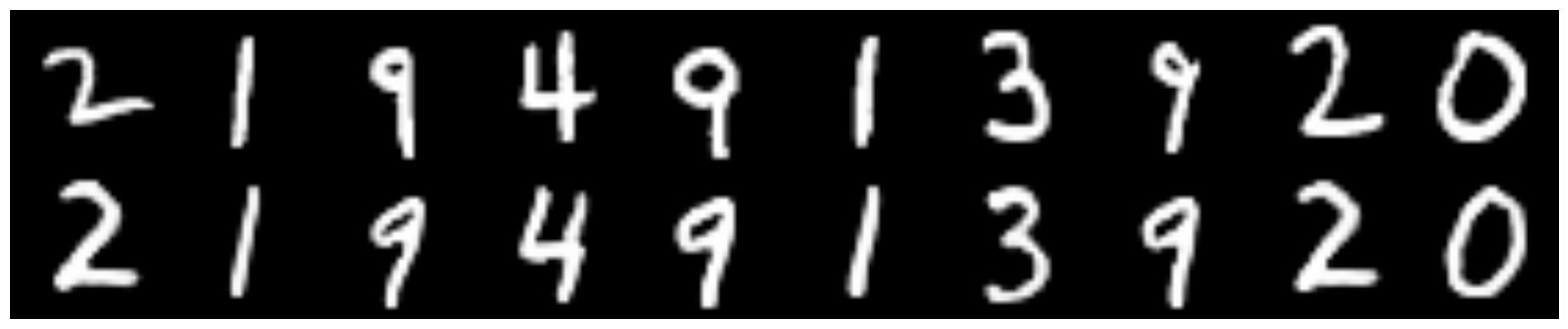
CVAE + GAN , hidden dimension - 8

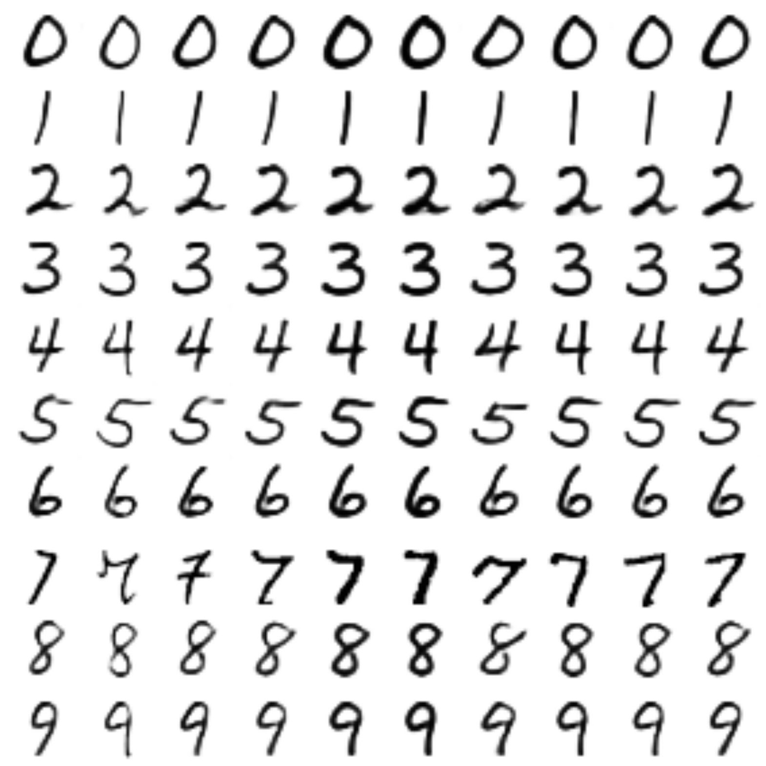
The generated digits of each label are sampled from N (0 | I)

Learning process

Gifs

Style transfer

The “7” was taken as a basis, from the style of which the rest of the figures were already created $\ dim Z = 8$ ).

So it was with a simple CVAE :

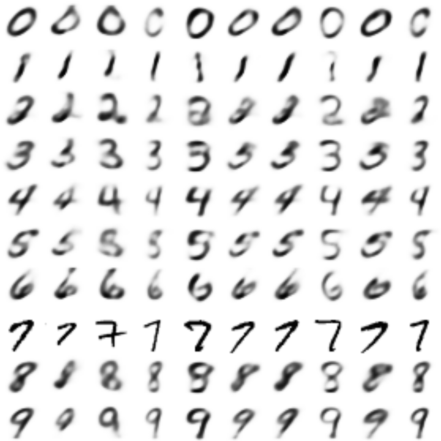
And so it became:

Conclusion

In my opinion, it turned out very well. Having gone from the simplest autoencoders , we reached generative models, namely, VAE , GAN , understood what conditional models are, and why the metric is important.
We also learned how to use keras and combine it with the bare tensorflow .

Thank you all for your attention, I hope it was interesting!

Repository with all laptops

Useful links and literature

Original article:
[1] Autoencoding beyond pixels using a learned similarity metric, Larsen et al, 2016, https://arxiv.org/abs/1512.09300

VAE Tutorial:
[2] Tutorial on Variational Autoencoders, Carl Doersch, 2016, https://arxiv.org/abs/1606.05908

Tutorial on using keras with tensorflow :
[3] https://blog.keras.io/keras-as-a-simplified-interface-to-tensorflow-tutorial.html

Source: https://habr.com/ru/post/332074/

All Articles

Autoencoders in Keras, Part 6: VAE + GAN

Content

We will understand in more detail why the recovered images are blurry.

Connecting VAE and GAN

Code

results

Comparison with a simple CVAE

Learning process

Style transfer

Conclusion

Useful links and literature

More articles: