Probabilistic and informational analysis of measurement results in Python

There is no more useful tool for research, than the theory confirmed by practice.

Why do we need information theory of measurements

In the previous publication [1] we considered the selection of the law of distribution of a random variable according to the statistical sampling data and only mentioned the informational approach to the analysis of measurement errors. Therefore, we will continue the discussion of this relevant topic.

The advantage of the informational approach to the analysis of measurement results is that the size of the entropy uncertainty interval can be found for any law of random error distribution. This eliminates "misunderstandings" with an arbitrary choice of values of confidence.
')
In addition, the set of probabilistic and informational characteristics of the sample can more accurately determine the nature of the distribution of random error. This is explained by the extensive base of the numerical values of such parameters as the entropy coefficient and the trajectory for various distribution laws and their superpositions.

On the essence of information and probabilistic analysis

Here the key word is uncertainty. Measurement is considered as a process, as a result of which the initial uncertainty in information about the measured value is reduced - x. A quantitative measure of uncertainty is entropy - H (x). More often, we encounter discrete values of the random variable x1, x2… xn, which is caused by the widespread use of computer technology. For such quantities, we write only one formula that explains a lot.

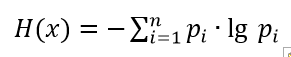(one)

Where p_i is the probability that the random variable x has taken the value x_i. Since 0≤p_i≤1, and while lg⁡p_i <0, then to obtain H (x) ≥0, the sum in the formula is a minus sign.

Entropy is measured in units of information. The information units on the above formula depend on the base of the logarithm. For the decimal logarithm, this is dit . For the natural logarithm - nit . For obvious reasons, the most frequently used binary logarithms are those at which entropy is measured in bits .

In the process of measurement, the initial uncertainty of x decreases as our knowledge of x increases. However, even after the measurement, the residual uncertainty H (∆) remains due to the measurement error ∆.

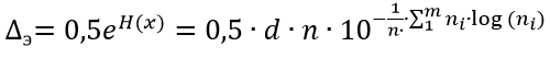
The residual entropy H (∆) can be determined by the above formula, substituting the error ∆ for x and, omitting the intermediate calculations, to obtain the entropy value of the error ∆ for any distribution law.

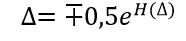(2)

How to get the entropy value of the error according to the measurement results

To do this, first the sequence of discrete values of the random variable of the error must be divided into intervals, followed by counting the frequencies of these values falling into each interval. Within the interval, the probability of the occurrence of these values of the error is assumed to be constant, equal to the ratio of the frequency of hitting this interval to the number of measurements taken.

In other words, you need to reproduce the part of the procedure that the hist () plotting function from the matplotlib library performs. Let us demonstrate this in the following simple procedure, comparing the resulting diagram with the diagram obtained with hist ().

Program for comparing data processing methods

import matplotlib.pyplot as plt import numpy as np from scipy.stats import uniform def diagram(a): a.sort()#   n=len(a)#     m= int(10+np.sqrt(n))#    d=(max(a)-min(a))/m#   x=[];y=[] for i in np.arange(0,m,1): x.append(min(a)+d*i)#      k=0 for j in a: if min(a)+d*i <=j<min(a)+d*(i+1): k=k+1 y.append(k)#         plt.title(" ") plt.bar(x,y, d) plt.grid(True) plt.show() plt.title("   hist()") plt.hist(a,m) plt.grid(True) plt.show() a=uniform.rvs(size=500) #     diagram(a)

Compare the resulting diagrams.

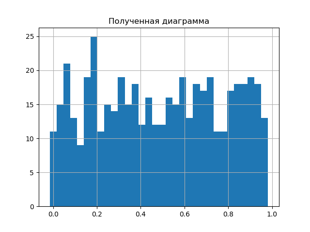
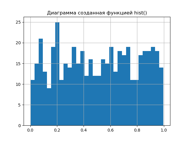
The diagrams are almost identical. A larger number by one than in the hist () function, the number of splitting intervals will only improve the result of the analysis. Therefore, we can proceed to the second stage of obtaining the entropy error value, for this we use the relation given in [2] and obtained from relation (2).

(3)

In the listing above, the list of x stores the values of the boundaries of the intervals, and the list of y contains the frequencies of the error values in these intervals. Rewrite (3) in the Python listing line.

h = 0.5 * d * n * 10 ** (-sum ([w * np.log10 (w) for w in y if w! = 0]) / n)

For the final solution of our problem, we will need two more values of the entropy coefficient k and the counter-process psi , we take them from [2], but we write them down for Python.

k = h / np.std (a)
mu4 = sum ([(w-np.mean (a)) ** 4 for w in a]) / n

It remains to add the four lines to the listing, but to analyze the final result, one more important question should be considered.

How can the entropy coefficient and counter-process be used to classify the error distribution laws

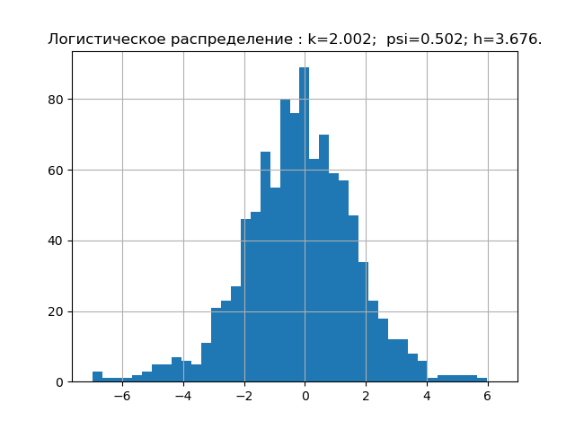
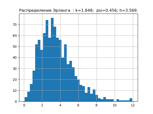
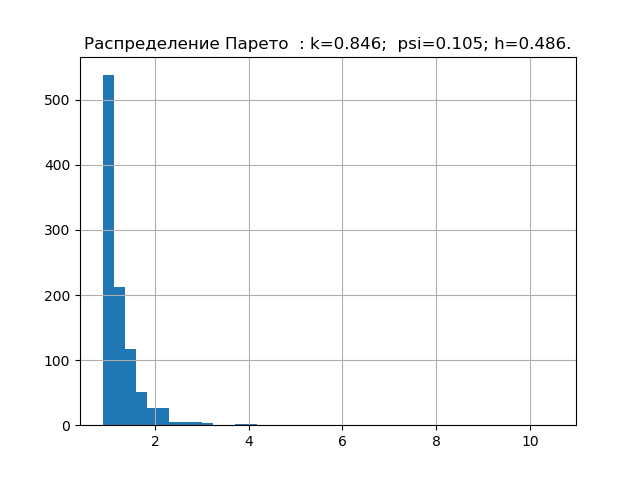
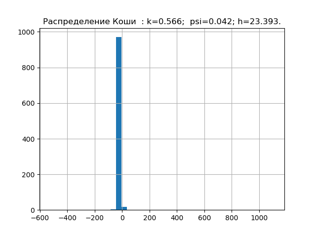
According to probability theory, the form of the distribution law is characterized by a relative fourth moment or a counter-process. In information theory, the form of the distribution law is determined by the value of the entropy coefficient. Taking this into account, we will place points on the psi, k plane corresponding to the given distribution laws. But first we obtain the values of psi, k and diagrams for the five most significant laws of the distribution of errors.

Program for obtaining numerical values of psi, k and plotting

 import matplotlib.pyplot as plt import numpy as np from scipy.stats import logistic,norm,uniform,erlang,pareto,cauchy def diagram(a,nr): a.sort() n=len(a) m= int(10+np.sqrt(n)) d=(max(a)-min(a))/m x=[];y=[] for i in np.arange(0,m,1): x.append(min(a)+d*i) k=0 for j in a: if min(a)+d*i <=j<min(a)+d*(i+1): k=k+1 y.append(k) h=0.5*d*n*10**(-sum([w*np.log10(w) for w in y if w!=0])/n) k=h/np.std (a) mu4=sum ([(w-np.mean (a))**4 for w in a])/n psi=(np.std(a))**2/np.sqrt(mu4) plt.title("%s : k=%s; psi=%s; h=%s."%(nr,str(round(k,3)),str(round(psi,3)),str(round(h,3)))) plt.bar(x,y, d) plt.grid(True) plt.show() nr=" " a=uniform.rvs( size=1000) diagram(a,nr) nr=" " a=logistic.rvs( size=1000) diagram(a,nr) nr=" " a=norm.rvs( size=1000) diagram(a,nr) nr="  " a = erlang.rvs(4,size=1000) diagram(a,nr) nr="  " a = pareto.rvs(4,size=1000) diagram(a,nr) nr="  " a = cauchy.rvs(size=1000) diagram(a,nr)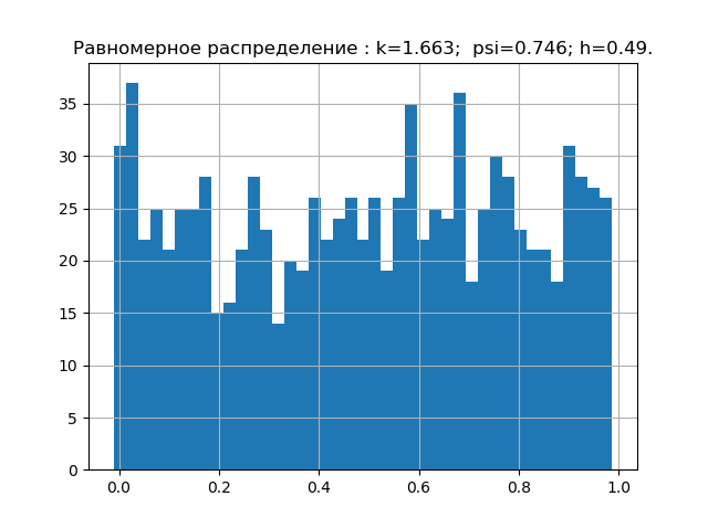

We have already accumulated the minimum base of entropy characteristics of the error distribution laws. Now let's check the theory on a sample with an unknown distribution law, for example, such.

a = [0.203, 0.154, 0.172, 0.192, 0.233, 0.181, 0.219, 0.153, 0.168, 0.132, 0.204, 0.165, 0.197, 0.205, 0.143, 0.201, 0.168, 0.147, 0.208, 0.195, 0.153, 0.193, 0.178, 0.162 , 0.157, 0.228, 0.219, 0.125, 0.101, 0.211, 0.183, 0.147, 0.145, 0.181, 0.184, 0.139, 0.198, 0.185, 0.202, 0.238, 0.167, 0.204, 0.195, 0.172, 0.196, 0.178, 0.113, 0.175, 0.194 , 0.178, 0.135, 0.178, 0.118, 0.186, 0.191]

If anyone is interested, you can choose any and check. This sample gives the following diagram with parameters.

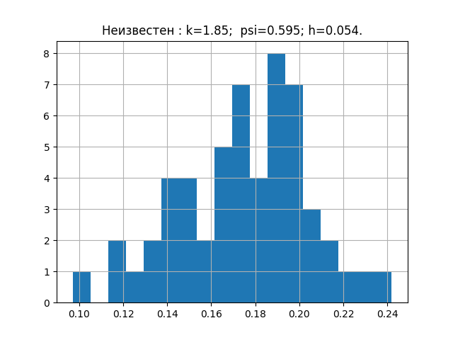
Now it's time to transfer the received parameters to the graph.

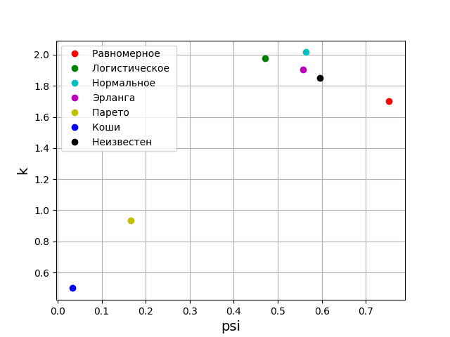
From the above graph it can be seen that the distribution law for the studied sample is closest to the Erlang distribution law.

Conclusion

I hope that the Python implementation of the elements of the information theory of measurements considered in this publication will not be uninteresting for you.

Thank you all for your attention!

Links

Source: https://habr.com/ru/post/332066/

All Articles