Autoencoders in Keras, Part 5: GAN (Generative Adversarial Networks) and tensorflow

Content

Part 1: Introduction
Part 2: Manifold learning and latent variables
Part 3: Variational autoencoders ( VAE )
Part 4: Conditional VAE
Part 5: GAN (Generative Adversarial Networks) and tensorflow
Part 6: VAE + GAN

(Because of yesterday's bug with perezalitami pictures on habrastoreydzh, which happened through no fault of mine, I was forced to remove this article yesterday immediately after publication. I post it again.)

With all the advantages of VAE variational autoencoders, which we dealt with in previous posts, they have one significant drawback: due to the poor way of comparing original and restored objects, the objects they generated are similar to the objects from the training set, but they are easily distinguishable from them (for example blurred).

This disadvantage is much less manifested in another approach, namely in generative competing networks - GAN 's.
')
Formally, GANs , of course, do not belong to autoencoders, however there are similarities between them and variational autoencoders, they will also be useful for the next part. So it will not be superfluous to meet them too.

GAN in brief

GAN 's were first proposed in [1, Generative Adversarial Nets, Goodfellow et al, 2014] and are now being actively studied. Most state-of-the-art generative models in one way or another use adversarial .

GAN scheme:

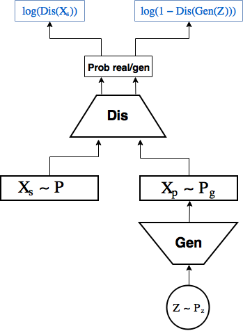
GAN 's consist of 2 neural networks:

1st — generator random samples from some given distribution , eg and generate objects from them $X_p = G (Z; \ theta_g)$ that go to the input of the second network,
2nd - the discriminator receives objects from the sample as input and created by the generator , and learns to predict the probability that a particular object is real, producing a scalar $D (X; \ theta_d)$ .

In this case, the generator trains to create objects that the discriminator does not distinguish from real ones.

Consider the GAN learning process.

The generator and the discriminator are trained separately, but within the same network.

Make k discriminator learning steps: per step discriminator learning parameters $\ theta_d$ updated to reduce cross-entropy:

$\ theta_d = \ theta_d - \ nabla _ {\ theta_d} \ left (\ log (D (X_s)) + \ log (1 - D (G (Z))) \ right)$

Next step generator training: update the parameters of the generator $\ theta_g$ in the direction of increasing the logarithm of the probability of the discriminator to assign the real label to the generated object.

$\ theta_g = \ theta_g + \ nabla _ {\ theta_g} \ log (1 - D (G (Z)))$

Training scheme:

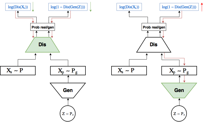
In the left picture the discriminator learning step: the gradient (red arrows) flows from the loss only to the discriminator, where they are updated $\ theta_d$ (green) in the direction of reducing the loss. In the right picture, the gradient from the right part of the loss (identification generated object identification error) flows to the generator, and only the generator weights are updated. $\ theta_g$ (green) in the direction of increasing the probability of the discriminator to be mistaken.

The task that the GAN solves is formulated as follows:

$\ min_G \ max_D \ mathbb {E} _ {X \ sim P} [\ log (D (X))] + \ mathbb {E} _ {Z \ sim P_z} [\ log (1 - D (G (Z )))]$

For a given generator, the optimal discriminator gives the probability $D ^ * (X) = \ frac {P (X)} {P_g (X) + P (X)},$ which is almost obvious, I suggest thinking about it for a second.

In [1] it is shown that with sufficient power of both networks, this task has an optimum, in which the generator learned to generate the distribution P_g (X)

matching with P (X)

, and everywhere on $X ^ {}$ discriminator gives probability 1/2

Illustration of [1]

Legend:

black dotted curve - true distribution ,
green - generator distribution ,
blue - probability distribution $D (X; \ theta_d)$ discriminator predict the class of a real object,
the lower and upper straight lines are the set of all and a lot of all , arrows represent mapping $G (Z; \ theta_g)$ .

On the picture:

(a) and quite different, but the discriminator uncertainly distinguishes one from the other,
(b) the discriminator after k learning steps already distinguishes them more confidently,
(c) it allows the generator guided by a good discriminator gradient , on the border of two distributions move closer to ,
(d) as a result of many repetitions of steps (a), (b), (c) coincided with and the discriminator is no longer able to distinguish one from the other: . Point optimum reached.

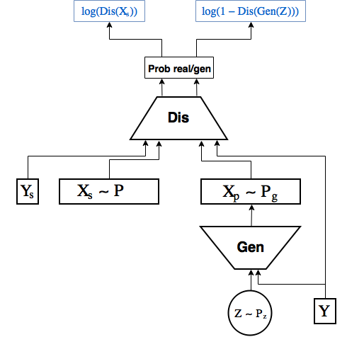
Conditional gan

Just like in the last part we made Conditional VAE , simply passing the numbers to the encoder and decoder label, here we will transfer it to the generator and the discriminator [2]

Code

Unlike the previous parts, where it was possible to manage with just one keras , there is a problem with this. Namely, it is necessary to update in turn one or only parameters of the generator, or only the discriminator in the same network. If you fake it, you can do it cleanly in keras , but for me it is easier and more useful to connect here and tensorflow .
The keras blog has a small tutorial [3] on how to do this.

The benefit of keras is easily combined with tensorflow - not for nothing, he got into tensorflow.contrib .

Let's start by importing the necessary modules and loading the dataset.

from IPython.display import clear_output import numpy as np import matplotlib.pyplot as plt %matplotlib inline from keras.layers import Dropout, BatchNormalization, Reshape, Flatten, RepeatVector from keras.layers import Lambda, Dense, Input, Conv2D, MaxPool2D, UpSampling2D, concatenate from keras.layers.advanced_activations import LeakyReLU from keras.models import Model, load_model from keras.datasets import mnist from keras.utils import to_categorical (x_train, y_train), (x_test, y_test) = mnist.load_data() x_train = x_train.astype('float32') / 255. x_test = x_test .astype('float32') / 255. x_train = np.reshape(x_train, (len(x_train), 28, 28, 1)) x_test = np.reshape(x_test, (len(x_test), 28, 28, 1)) y_train_cat = to_categorical(y_train).astype(np.float32) y_test_cat = to_categorical(y_test).astype(np.float32)

To work in keras and tensorflow, you need to simultaneously register a tensorflow session in keras , it is necessary for keras to create all internal variables within the session used.

 from keras import backend as K import tensorflow as tf sess = tf.Session() K.set_session(sess)

Define the main global constants:

 batch_size = 256 batch_shape = (batch_size, 28, 28, 1) latent_dim = 2 num_classes = 10 dropout_rate = 0.3

Now we will not train the model using the .fit method, but directly from tensorflow , so we will write an iterator that returns the next batch:

 def gen_batch(x, y): n_batches = x.shape[0] // batch_size while(True): for i in range(n_batches): yield x[batch_size*i: batch_size*(i+1)], y[batch_size*i: batch_size*(i+1)] idxs = np.random.permutation(y.shape[0]) x = x[idxs] y = y[idxs] train_batches_it = gen_batch(x_train, y_train_cat) test_batches_it = gen_batch(x_test, y_test_cat)

Wrap placeholder 's for images, labels, and hidden variables in the incoming layers for keras models:

 x_ = tf.placeholder(tf.float32, shape=(None, 28, 28, 1), name='image') y_ = tf.placeholder(tf.float32, shape=(None, num_classes), name='labels') z_ = tf.placeholder(tf.float32, shape=(None, latent_dim), name='z') img = Input(tensor=x_) lbl = Input(tensor=y_) z = Input(tensor=z_)

We will implement CGAN immediately, as it is only minimally different from the usual.
We write a model of the generator. Keras works with scope , and we need to separate the generator and the discriminator in order to train them separately

 with tf.variable_scope('generator'): x = concatenate([z, lbl]) x = Dense(7*7*64, activation='relu')(x) x = Dropout(dropout_rate)(x) x = Reshape((7, 7, 64))(x) x = UpSampling2D(size=(2, 2))(x) x = Conv2D(64, kernel_size=(5, 5), activation='relu', padding='same')(x) x = Dropout(dropout_rate)(x) x = Conv2D(32, kernel_size=(3, 3), activation='relu', padding='same')(x) x = Dropout(dropout_rate)(x) x = UpSampling2D(size=(2, 2))(x) generated = Conv2D(1, kernel_size=(5, 5), activation='sigmoid', padding='same')(x) generator = Model([z, lbl], generated, name='generator')

Further, the discriminator model. Here we need to add another label to the incoming image. To do this, after applying the first convolutional layer, add labels to the filters. First, the function that does it, then the discriminator model.

 def add_units_to_conv2d(conv2, units): dim1 = int(conv2.shape[1]) dim2 = int(conv2.shape[2]) dimc = int(units.shape[1]) repeat_n = dim1*dim2 units_repeat = RepeatVector(repeat_n)(lbl) units_repeat = Reshape((dim1, dim2, dimc))(units_repeat) return concatenate([conv2, units_repeat]) with tf.variable_scope('discrim'): x = Conv2D(128, kernel_size=(7, 7), strides=(2, 2), padding='same')(img) x = add_units_to_conv2d(x, lbl) x = LeakyReLU()(x) x = Dropout(dropout_rate)(x) x = MaxPool2D((2, 2), padding='same')(x) l = Conv2D(128, kernel_size=(3, 3), padding='same')(x) x = LeakyReLU()(l) x = Dropout(dropout_rate)(x) h = Flatten()(x) d = Dense(1, activation='sigmoid')(h) discrim = Model([img, lbl], d, name='Discriminator')

Having defined models, we can apply them directly to place holders as ordinary tensorflow operations.

 generated_z = generator([z, lbl]) discr_img = discrim([img, lbl]) discr_gen_z = discrim([generated_z, lbl]) gan_model = Model([z, lbl], discr_gen_z, name='GAN') gan = gan_model([z, lbl])

Now the loss is the error of determining the real image, and the loss generated by, as well as on the basis of, the losses of the generator and discriminator.

 log_dis_img = tf.reduce_mean(-tf.log(discr_img + 1e-10)) log_dis_gen_z = tf.reduce_mean(-tf.log(1. - discr_gen_z + 1e-10)) L_gen = -log_dis_gen_z L_dis = 0.5*(log_dis_gen_z + log_dis_img)

Usually in tensorflow , passing to the optimizer a loss, it will try to minimize all the variables on which it depends. We do not need this now: when training a generator, the error should not touch the discriminator, although it should flow through it and vice versa.

To do this, in addition to the optimizer, you must pass a list of variables that it will optimize. We will get these variables from the required scope using tf.get_collection

 optimizer_gen = tf.train.RMSPropOptimizer(0.0003) optimizer_dis = tf.train.RMSPropOptimizer(0.0001) #     ()   generator_vars = tf.get_collection(tf.GraphKeys.TRAINABLE_VARIABLES, "generator") discrim_vars = tf.get_collection(tf.GraphKeys.TRAINABLE_VARIABLES, "discrim") step_gen = optimizer_gen.minimize(L_gen, var_list=generator_vars) step_dis = optimizer_dis.minimize(L_dis, var_list=discrim_vars)

Initialize the variables:

 sess.run(tf.global_variables_initializer())

Separately, we will write the functions that we will call to train the generator and the discriminator:

 #    def step(image, label, zp): l_dis, _ = sess.run([L_dis, step_gen], feed_dict={z:zp, lbl:label, img:image, K.learning_phase():1}) return l_dis #    def step_d(image, label, zp): l_dis, _ = sess.run([L_dis, step_dis], feed_dict={z:zp, lbl:label, img:image, K.learning_phase():1}) return l_dis

Code saving and visualization of images:

Code

 # ,     ,    figs = [[] for x in range(num_classes)] periods = [] save_periods = list(range(100)) + list(range(100, 1000, 10)) n = 15 #   15x15  from scipy.stats import norm #     N(0, I),   ,    ,      grid_x = norm.ppf(np.linspace(0.05, 0.95, n)) grid_y = norm.ppf(np.linspace(0.05, 0.95, n)) grid_y = norm.ppf(np.linspace(0.05, 0.95, n)) def draw_manifold(label, show=True): #     figure = np.zeros((28 * n, 28 * n)) input_lbl = np.zeros((1, 10)) input_lbl[0, label] = 1. for i, yi in enumerate(grid_x): for j, xi in enumerate(grid_y): z_sample = np.zeros((1, latent_dim)) z_sample[:, :2] = np.array([[xi, yi]]) x_generated = sess.run(generated_z, feed_dict={z:z_sample, lbl:input_lbl, K.learning_phase():0}) digit = x_generated[0].squeeze() figure[i * 28: (i + 1) * 28, j * 28: (j + 1) * 28] = digit if show: #  plt.figure(figsize=(10, 10)) plt.imshow(figure, cmap='Greys') plt.grid(False) ax = plt.gca() ax.get_xaxis().set_visible(False) ax.get_yaxis().set_visible(False) plt.show() return figure n_compare = 10 def on_n_period(period): clear_output() #   output #     y draw_lbl = np.random.randint(0, num_classes) print(draw_lbl) for label in range(num_classes): figs[label].append(draw_manifold(label, show=label==draw_lbl)) periods.append(period)

Now we will train our CGAN .

It is important that at the very beginning the discriminator does not begin to win too much, otherwise the learning will stop. Therefore, internal cycles are added here both for the discriminator and for the generator, and the output from them, when one network almost catches up with another.

If the discriminator immediately wins the decoder, and the training does not even have time to start, then you can try to slow down the discriminator’s training or start anew several times.

 batches_per_period = 20 #     k_step = 5 #  ,          for i in range(5000): print('.', end='') #    b0, b1 = next(train_batches_it) zp = np.random.randn(batch_size, latent_dim) #    for j in range(k_step): l_d = step_d(b0, b1, zp) b0, b1 = next(train_batches_it) zp = np.random.randn(batch_size, latent_dim) if l_d < 1.0: break #    for j in range(k_step): l_d = step(b0, b1, zp) if l_d > 0.4: break b0, b1 = next(train_batches_it) zp = np.random.randn(batch_size, latent_dim) #    if not i % batches_per_period: period = i // batches_per_period if period in save_periods: on_n_period(period) print(l_d)

Gif drawing code:

Code

 from matplotlib.animation import FuncAnimation from matplotlib import cm import matplotlib def make_2d_figs_gif(figs, periods, c, fname, fig, batches_per_period): norm = matplotlib.colors.Normalize(vmin=0, vmax=1, clip=False) im = plt.imshow(np.zeros((28,28)), cmap='Greys', norm=norm) plt.grid(None) plt.title("Label: {}\nBatch: {}".format(c, 0)) def update(i): im.set_array(figs[i]) im.axes.set_title("Label: {}\nBatch: {}".format(c, periods[i]*batches_per_period)) im.axes.get_xaxis().set_visible(False) im.axes.get_yaxis().set_visible(False) return im anim = FuncAnimation(fig, update, frames=range(len(figs)), interval=100) anim.save(fname, dpi=80, writer='imagemagick') for label in range(num_classes): make_2d_figs_gif(figs[label], periods, label, "./figs4_5/manifold_{}.gif".format(label), plt.figure(figsize=(10,10)), batches_per_period)

Results:

Gan

Variety digits for regular GAN (without label transfer)

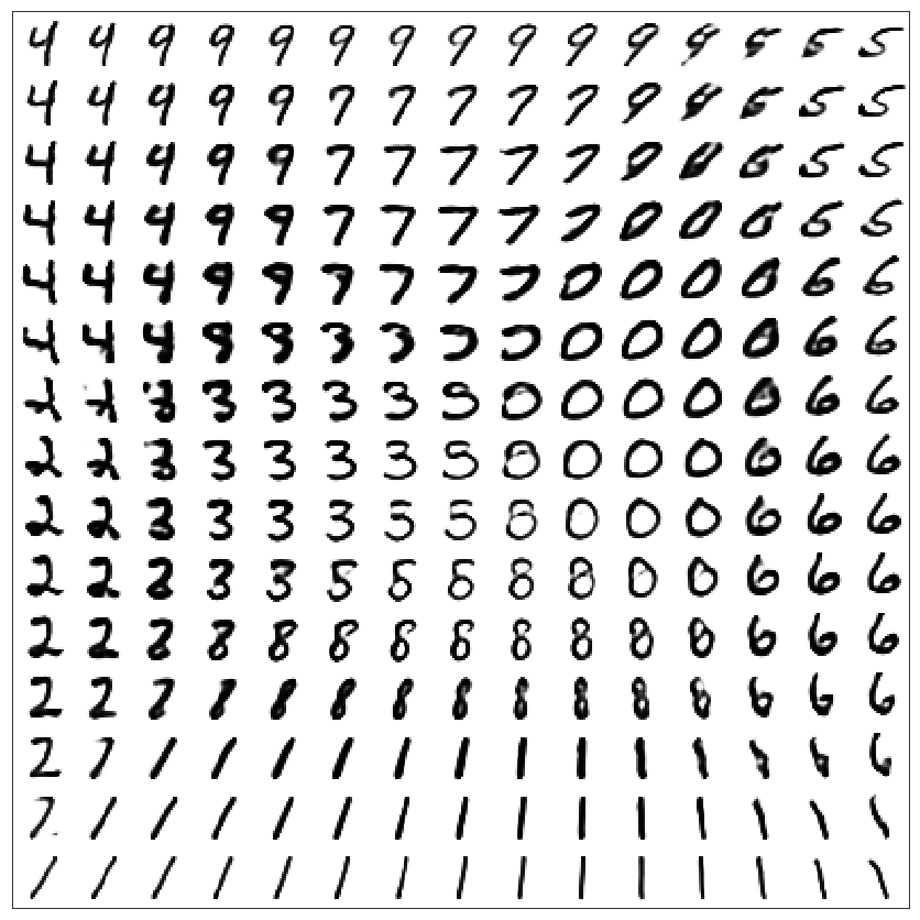
It is worth noting that the numbers are better than in VAE (without labels)

Learning gif

CGAN

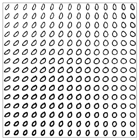
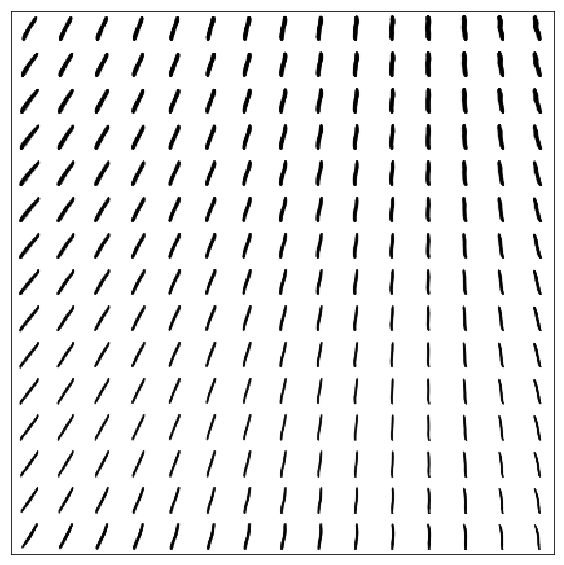
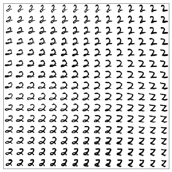
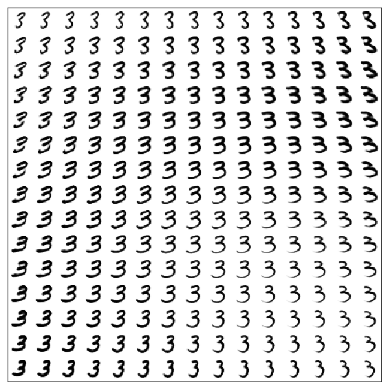
Varieties of numbers for each label

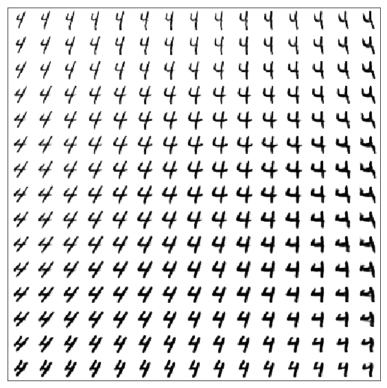
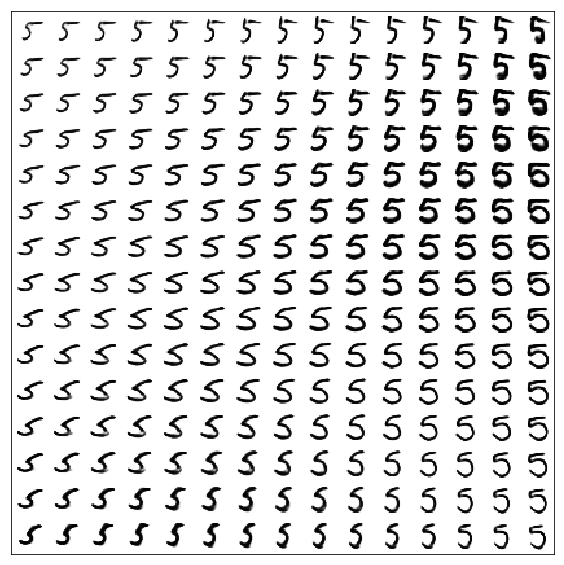
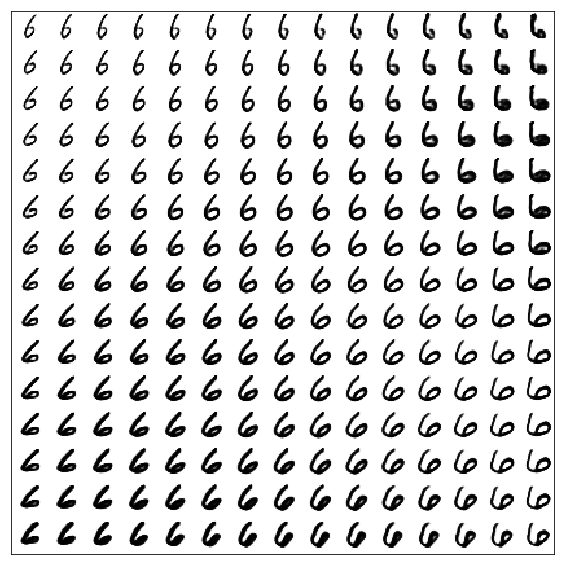
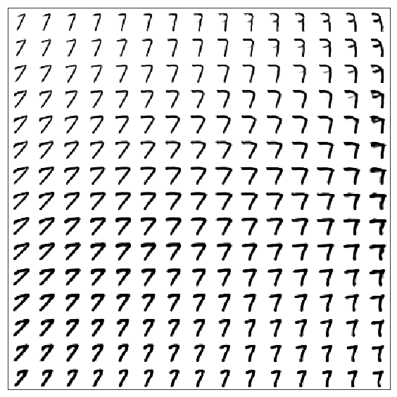
Heavy gifs

Useful links and literature

Original article:
[1] Generative Adversarial Nets, Goodfellow et al, 2014, https://arxiv.org/abs/1406.2661

Conditional GANs:
[2] Conditional Generative Adversarial Nets, Mirza, Osindero, 2014, https://arxiv.org/abs/1411.1784

Tutorial about using keras with tensorflow :
[3] https://blog.keras.io/keras-as-a-simplified-interface-to-tensorflow-tutorial.html

Source: https://habr.com/ru/post/332000/

All Articles