Autoencoders in Keras, Part 4: Conditional VAE
Content
- Part 1: Introduction
- Part 2: Manifold learning and latent variables
- Part 3: Variational autoencoders ( VAE )
- Part 4: Conditional VAE
- Part 5: GAN (Generative Adversarial Networks) and tensorflow
- Part 6: VAE + GAN
In the last part, we met variational autoencoders (VAE) , implemented one on keras , and also understood how to generate images using it. The resulting model, however, had some drawbacks:
- Not all the numbers turned out to be well encoded in the hidden space: some of the numbers were either completely absent or were very blurry. In between the areas in which the variants of the same figure were concentrated, there were generally some meaningless hieroglyphs.
What is there to write, this is how the generated numbers looked like:
')Picture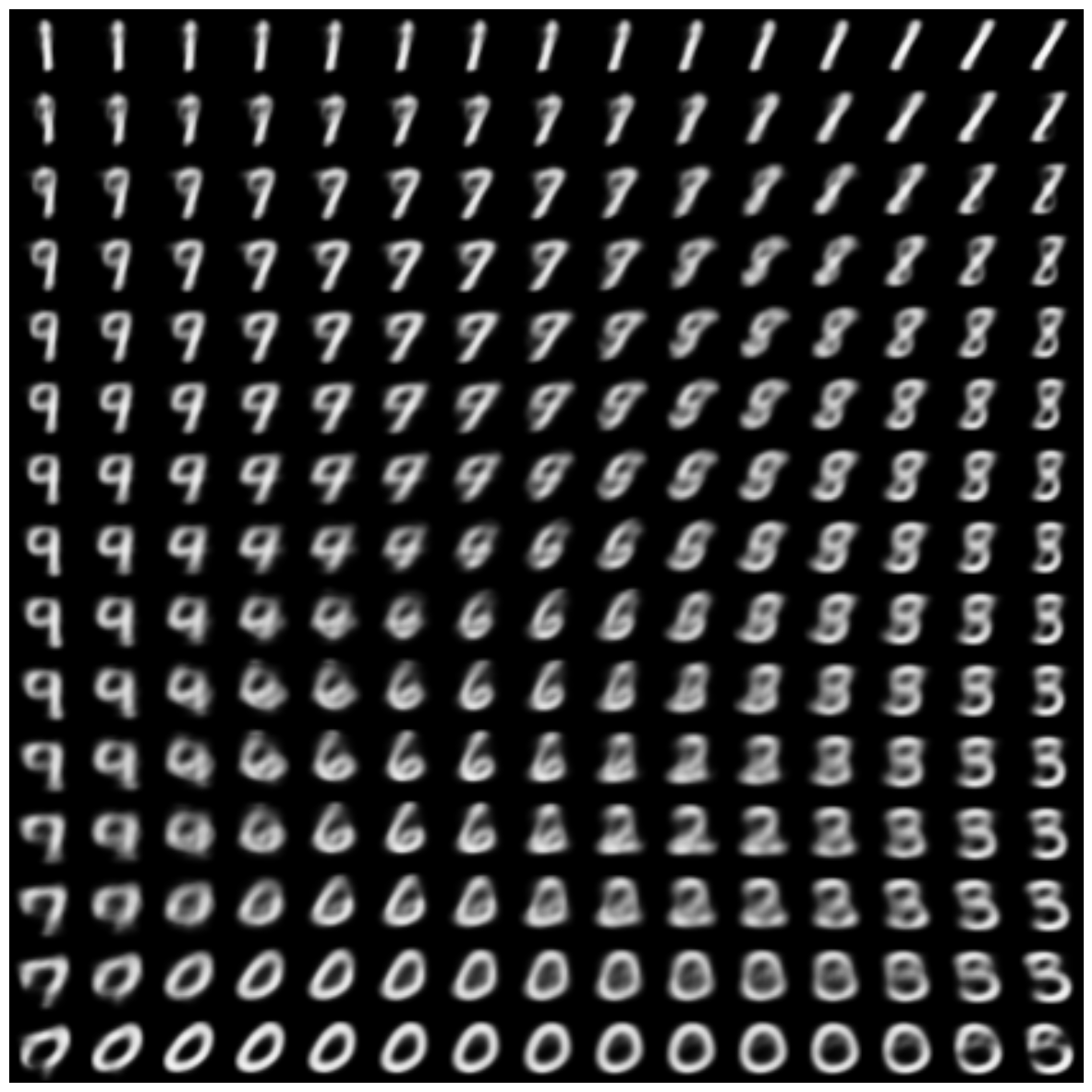
- It was difficult to generate a picture of a given digit. To do this, it was necessary to look into what area of the latent space the images of a particular digit fell into, and to sample it from somewhere, and even more so it was difficult to generate a digit in some given style.
In this part, we will see how only by slightly complicating the model to overcome both these problems, and at the same time we will be able to generate pictures of new numbers in the style of another digit - this is probably the most interesting feature of the future model.
At first we will think about the reasons for the 1st shortcoming:
The varieties on which different numbers lie can be far apart in the space of pictures. That is, it is difficult to imagine how, for example, to continuously display a picture of the number “5”, into a picture of the number “7”, while all the intermediate pictures could be called plausible. Thus, the variety, near which the numbers lie, does not necessarily have to be linearly connected. The autoencoder, due to the fact that it is a composition of continuous functions, can itself be displayed in the code and back only continuously, especially if it is a variational autoencoder. In our previous example, the situation was further complicated by the fact that the autoencoder tried to search for a two-dimensional manifold.
As an illustration, let us return to our artificial example from the 2nd part, just make the defining manifold disconnected:
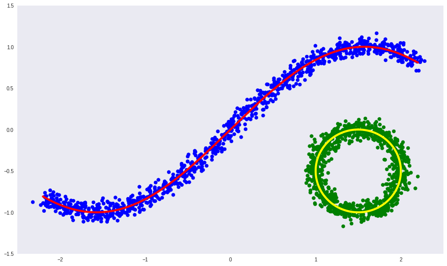
Here:
- blue and green dots are sampled objects,
- red and yellow curves - unrelated defining manifold.
Let us now try to learn the defining variety using the usual deep autoencoder.
Code
# import numpy as np import matplotlib.pyplot as plt %matplotlib inline import seaborn as sns # x1 = np.linspace(-2.2, 2.2, 1000) fx = np.sin(x1) dots1 = np.vstack([x1, fx]).T t = np.linspace(0, 2*np.pi, num=1000) dots2 = 0.5*np.array([np.sin(t), np.cos(t)]).T + np.array([1.5, -0.5])[None, :] dots = np.vstack([dots1, dots2]) noise = 0.06 * np.random.randn(*dots.shape) labels = np.array([0]*1000 + [1]*1000) noised = dots + noise # colors = ['b']*1000 + ['g']*1000 plt.figure(figsize=(15, 9)) plt.xlim([-2.5, 2.5]) plt.ylim([-1.5, 1.5]) plt.scatter(noised[:, 0], noised[:, 1], c=colors) plt.plot(dots1[:, 0], dots1[:, 1], color="red", linewidth=4) plt.plot(dots2[:, 0], dots2[:, 1], color="yellow", linewidth=4) plt.grid(False) # from keras.layers import Input, Dense from keras.models import Model from keras.optimizers import Adam def deep_ae(): input_dots = Input((2,)) x = Dense(64, activation='elu')(input_dots) x = Dense(64, activation='elu')(x) code = Dense(1, activation='linear')(x) x = Dense(64, activation='elu')(code) x = Dense(64, activation='elu')(x) out = Dense(2, activation='linear')(x) ae = Model(input_dots, out) return ae dae = deep_ae() dae.compile(Adam(0.001), 'mse') dae.fit(noised, noised, epochs=300, batch_size=30, verbose=2) # predicted = dae.predict(noised) # plt.figure(figsize=(15, 9)) plt.xlim([-2.5, 2.5]) plt.ylim([-1.5, 1.5]) plt.scatter(noised[:, 0], noised[:, 1], c=colors) plt.plot(dots1[:, 0], dots1[:, 1], color="red", linewidth=4) plt.plot(dots2[:, 0], dots2[:, 1], color="yellow", linewidth=4) plt.scatter(predicted[:, 0], predicted[:, 1], c='white', s=50) plt.grid(False) 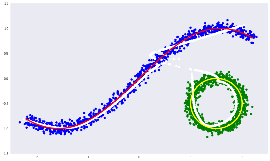
- the white line is the manifold into which the blue and green data points pass after the autoencoder, that is, the autoencoder's attempt to construct the manifold that determines the most variation in the data.
It can be seen that a simple autoencoder failed to learn the shape of a disconnected manifold. Instead, he slyly continued one another.
If we know the data labels, which determine on which of the parts of the disconnected manifold these data lie (as with the numbers), then we can simply condition the autoencoder on these labels. That is, just additionally with the data to feed the data to the encoder and the decoder as well. In this case, the source of discontinuities in the data will be the label, and this will allow the autoencoder to learn each part of a linearly disconnected manifold separately.
Let's look at the same example, only now we will transfer the label to the input and the encoder and the decoder additionally.
Code
from keras.layers import concatenate def deep_cond_ae(): input_dots = Input((2,)) input_lbls = Input((1,)) full_input = concatenate([input_dots, input_lbls]) x = Dense(64, activation='elu')(full_input) x = Dense(64, activation='elu')(x) code = Dense(1, activation='linear')(x) full_code = concatenate([code, input_lbls]) x = Dense(64, activation='elu')(full_code) x = Dense(64, activation='elu')(x) out = Dense(2, activation='linear')(x) ae = Model([input_dots, input_lbls], out) return ae cdae = deep_cond_ae() cdae.compile(Adam(0.001), 'mse') cdae.fit([noised, labels], noised, epochs=300, batch_size=30, verbose=2) predicted = cdae.predict([noised, labels]) # plt.figure(figsize=(15, 9)) plt.xlim([-2.5, 2.5]) plt.ylim([-1.5, 1.5]) plt.scatter(noised[:, 0], noised[:, 1], c=colors) plt.plot(dots1[:, 0], dots1[:, 1], color="red", linewidth=4) plt.plot(dots2[:, 0], dots2[:, 1], color="yellow", linewidth=4) plt.scatter(predicted[:, 0], predicted[:, 1], c='white', s=50) plt.grid(False) 
This time, the autoencoder managed to learn a linearly disconnected defining manifold.
CVAE
If you now take the VAE , as in the previous part, and also feed labels to the input, you get a Conditional Variational Autoencoder (CVAE) .
With pictures of numbers it turns out like this:

Picture above from [2]
In this case, the VAE basic equation from the last part becomes simply conditioned on
 ( not required to be discrete), that is, on the label.
![\ log P (X | Y; \ theta_2) - KL [Q (Z | X, Y; \ theta_1) || P (Z | X, Y; \ theta_2)] = E_ {Z \ sim Q} [\ log P (X | Z, Y; \ theta_2)] - KL [Q (Z | X, Y; \ theta_1) || N (0, I)]](https://habrastorage.org/getpro/habr/post_images/2a6/61b/69e/2a661b69ea2aa2351f7493a41469c789.svg)
 we again compare with
  .
.This can be interpreted as: for each
we have a separate VAE autoencoder, while they have a huge amount of common weights (almost absolute weight sharing ).The result is that CVAE codes in
 input signal properties common to all .
Style transfer
(Comment: this is not the same thing as transferring the style to Prisme, there is something else entirely)
Now it becomes clear how to create new images in the style given:
- we train CVAE on pictures with labels,
- we encode the style of the given picture in ,
- changing labels create from coded new pictures.
Keras code
The code is almost identical to the code from the previous part, except that now the label of the digit is transmitted to the encoder and the decoder.
Code
import sys import numpy as np import matplotlib.pyplot as plt %matplotlib inline # import seaborn as sns from keras.datasets import mnist from keras.utils import to_categorical (x_train, y_train), (x_test, y_test) = mnist.load_data() x_train = x_train.astype('float32') / 255. x_test = x_test .astype('float32') / 255. x_train = np.reshape(x_train, (len(x_train), 28, 28, 1)) x_test = np.reshape(x_test, (len(x_test), 28, 28, 1)) y_train_cat = to_categorical(y_train).astype(np.float32) y_test_cat = to_categorical(y_test).astype(np.float32) num_classes = y_test_cat.shape[1] batch_size = 500 latent_dim = 8 dropout_rate = 0.3 start_lr = 0.001 from keras.layers import Input, Dense from keras.layers import BatchNormalization, Dropout, Flatten, Reshape, Lambda from keras.layers import concatenate from keras.models import Model from keras.objectives import binary_crossentropy from keras.layers.advanced_activations import LeakyReLU from keras import backend as K def create_cvae(): models = {} # Dropout BatchNormalization def apply_bn_and_dropout(x): return Dropout(dropout_rate)(BatchNormalization()(x)) # input_img = Input(shape=(28, 28, 1)) flatten_img = Flatten()(input_img) input_lbl = Input(shape=(num_classes,), dtype='float32') x = concatenate([flatten_img, input_lbl]) x = Dense(256, activation='relu')(x) x = apply_bn_and_dropout(x) # # , z_mean = Dense(latent_dim)(x) z_log_var = Dense(latent_dim)(x) # Q def sampling(args): z_mean, z_log_var = args epsilon = K.random_normal(shape=(batch_size, latent_dim), mean=0., stddev=1.0) return z_mean + K.exp(z_log_var / 2) * epsilon l = Lambda(sampling, output_shape=(latent_dim,))([z_mean, z_log_var]) models["encoder"] = Model([input_img, input_lbl], l, 'Encoder') models["z_meaner"] = Model([input_img, input_lbl], z_mean, 'Enc_z_mean') models["z_lvarer"] = Model([input_img, input_lbl], z_log_var, 'Enc_z_log_var') # z = Input(shape=(latent_dim, )) input_lbl_d = Input(shape=(num_classes,), dtype='float32') x = concatenate([z, input_lbl_d]) x = Dense(256)(x) x = LeakyReLU()(x) x = apply_bn_and_dropout(x) x = Dense(28*28, activation='sigmoid')(x) decoded = Reshape((28, 28, 1))(x) models["decoder"] = Model([z, input_lbl_d], decoded, name='Decoder') models["cvae"] = Model([input_img, input_lbl, input_lbl_d], models["decoder"]([models["encoder"]([input_img, input_lbl]), input_lbl_d]), name="CVAE") models["style_t"] = Model([input_img, input_lbl, input_lbl_d], models["decoder"]([models["z_meaner"]([input_img, input_lbl]), input_lbl_d]), name="style_transfer") def vae_loss(x, decoded): x = K.reshape(x, shape=(batch_size, 28*28)) decoded = K.reshape(decoded, shape=(batch_size, 28*28)) xent_loss = 28*28*binary_crossentropy(x, decoded) kl_loss = -0.5 * K.sum(1 + z_log_var - K.square(z_mean) - K.exp(z_log_var), axis=-1) return (xent_loss + kl_loss)/2/28/28 return models, vae_loss models, vae_loss = create_cvae() cvae = models["cvae"] from keras.optimizers import Adam, RMSprop cvae.compile(optimizer=Adam(start_lr), loss=vae_loss) digit_size = 28 def plot_digits(*args, invert_colors=False): args = [x.squeeze() for x in args] n = min([x.shape[0] for x in args]) figure = np.zeros((digit_size * len(args), digit_size * n)) for i in range(n): for j in range(len(args)): figure[j * digit_size: (j + 1) * digit_size, i * digit_size: (i + 1) * digit_size] = args[j][i].squeeze() if invert_colors: figure = 1-figure plt.figure(figsize=(2*n, 2*len(args))) plt.imshow(figure, cmap='Greys_r') plt.grid(False) ax = plt.gca() ax.get_xaxis().set_visible(False) ax.get_yaxis().set_visible(False) plt.show() n = 15 # 15x15 from scipy.stats import norm # N(0, I), , , grid_x = norm.ppf(np.linspace(0.05, 0.95, n)) grid_y = norm.ppf(np.linspace(0.05, 0.95, n)) def draw_manifold(generator, lbl, show=True): # figure = np.zeros((digit_size * n, digit_size * n)) input_lbl = np.zeros((1, 10)) input_lbl[0, lbl] = 1 for i, yi in enumerate(grid_x): for j, xi in enumerate(grid_y): z_sample = np.zeros((1, latent_dim)) z_sample[:, :2] = np.array([[xi, yi]]) x_decoded = generator.predict([z_sample, input_lbl]) digit = x_decoded[0].squeeze() figure[i * digit_size: (i + 1) * digit_size, j * digit_size: (j + 1) * digit_size] = digit if show: # plt.figure(figsize=(10, 10)) plt.imshow(figure, cmap='Greys_r') plt.grid(False) ax = plt.gca() ax.get_xaxis().set_visible(False) ax.get_yaxis().set_visible(False) plt.show() return figure def draw_z_distr(z_predicted, lbl): # z input_lbl = np.zeros((1, 10)) input_lbl[0, lbl] = 1 im = plt.scatter(z_predicted[:, 0], z_predicted[:, 1]) im.axes.set_xlim(-5, 5) im.axes.set_ylim(-5, 5) plt.show() from IPython.display import clear_output from keras.callbacks import LambdaCallback, ReduceLROnPlateau, TensorBoard # , figs = [[] for x in range(num_classes)] latent_distrs = [[] for x in range(num_classes)] epochs = [] # , save_epochs = set(list((np.arange(0, 59)**1.701).astype(np.int)) + list(range(10))) # imgs = x_test[:batch_size] imgs_lbls = y_test_cat[:batch_size] n_compare = 10 # generator = models["decoder"] encoder_mean = models["z_meaner"] # , def on_epoch_end(epoch, logs): if epoch in save_epochs: clear_output() # output # decoded = cvae.predict([imgs, imgs_lbls, imgs_lbls], batch_size=batch_size) plot_digits(imgs[:n_compare], decoded[:n_compare]) # y z|y draw_lbl = np.random.randint(0, num_classes) print(draw_lbl) for lbl in range(num_classes): figs[lbl].append(draw_manifold(generator, lbl, show=lbl==draw_lbl)) idxs = y_test == lbl z_predicted = encoder_mean.predict([x_test[idxs], y_test_cat[idxs]], batch_size) latent_distrs[lbl].append(z_predicted) if lbl==draw_lbl: draw_z_distr(z_predicted, lbl) epochs.append(epoch) # pltfig = LambdaCallback(on_epoch_end=on_epoch_end) # lr_red = ReduceLROnPlateau(factor=0.1, patience=25) tb = TensorBoard(log_dir='./logs') # cvae.fit([x_train, y_train_cat, y_train_cat], x_train, shuffle=True, epochs=1000, batch_size=batch_size, validation_data=([x_test, y_test_cat, y_test_cat], x_test), callbacks=[pltfig, tb], verbose=1) results
(I apologize that in some places there are white numbers on a black background, and in some places black on white)
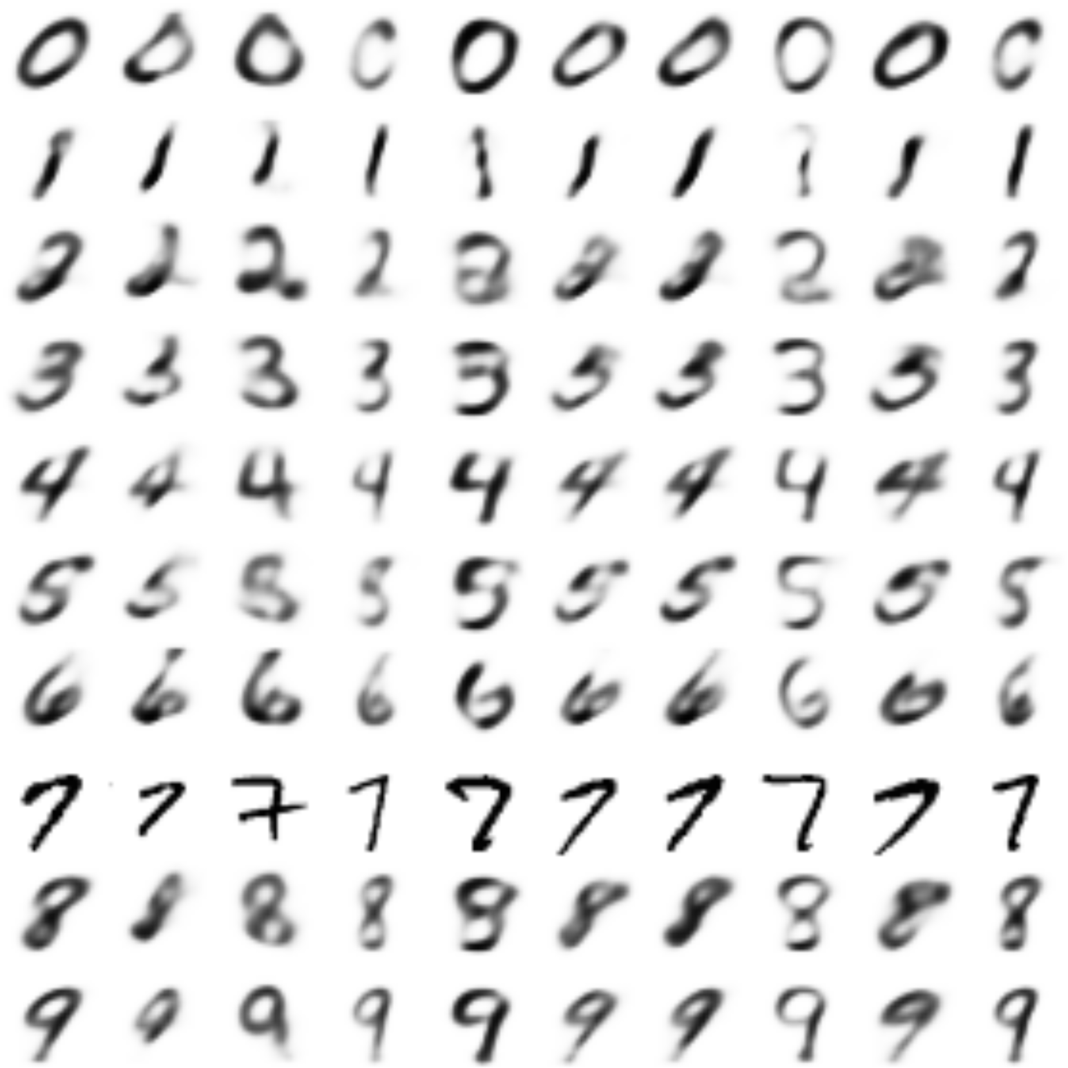
This autoencoder translates numbers like this:

The generated digits of each label are sampled from
 :
:(It is perfectly visible how common features are coded in coordinates
)

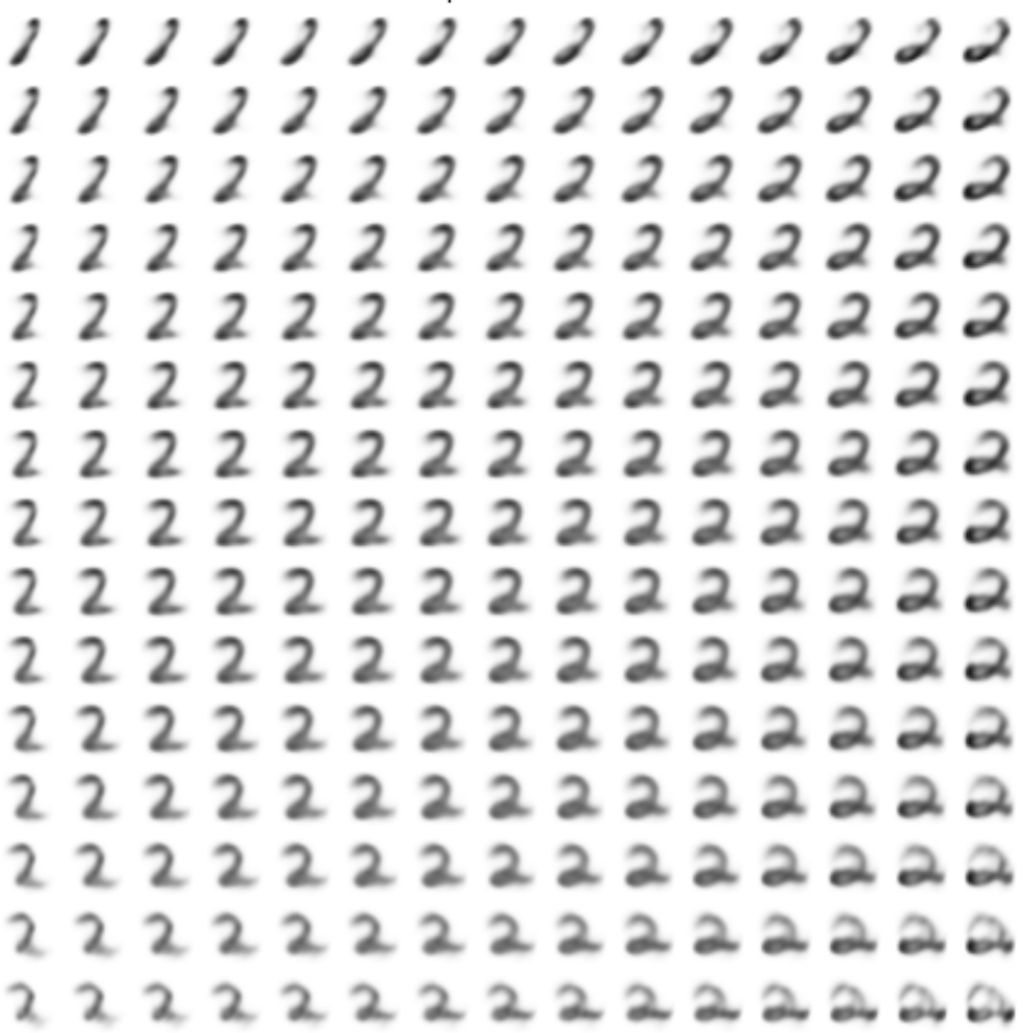
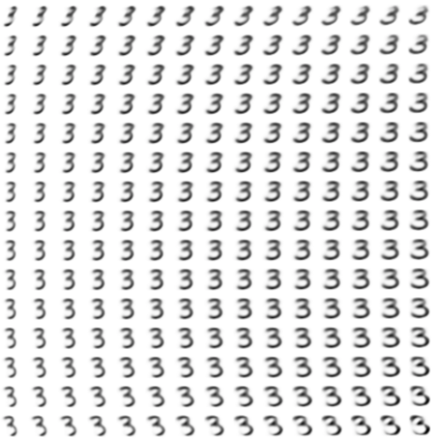
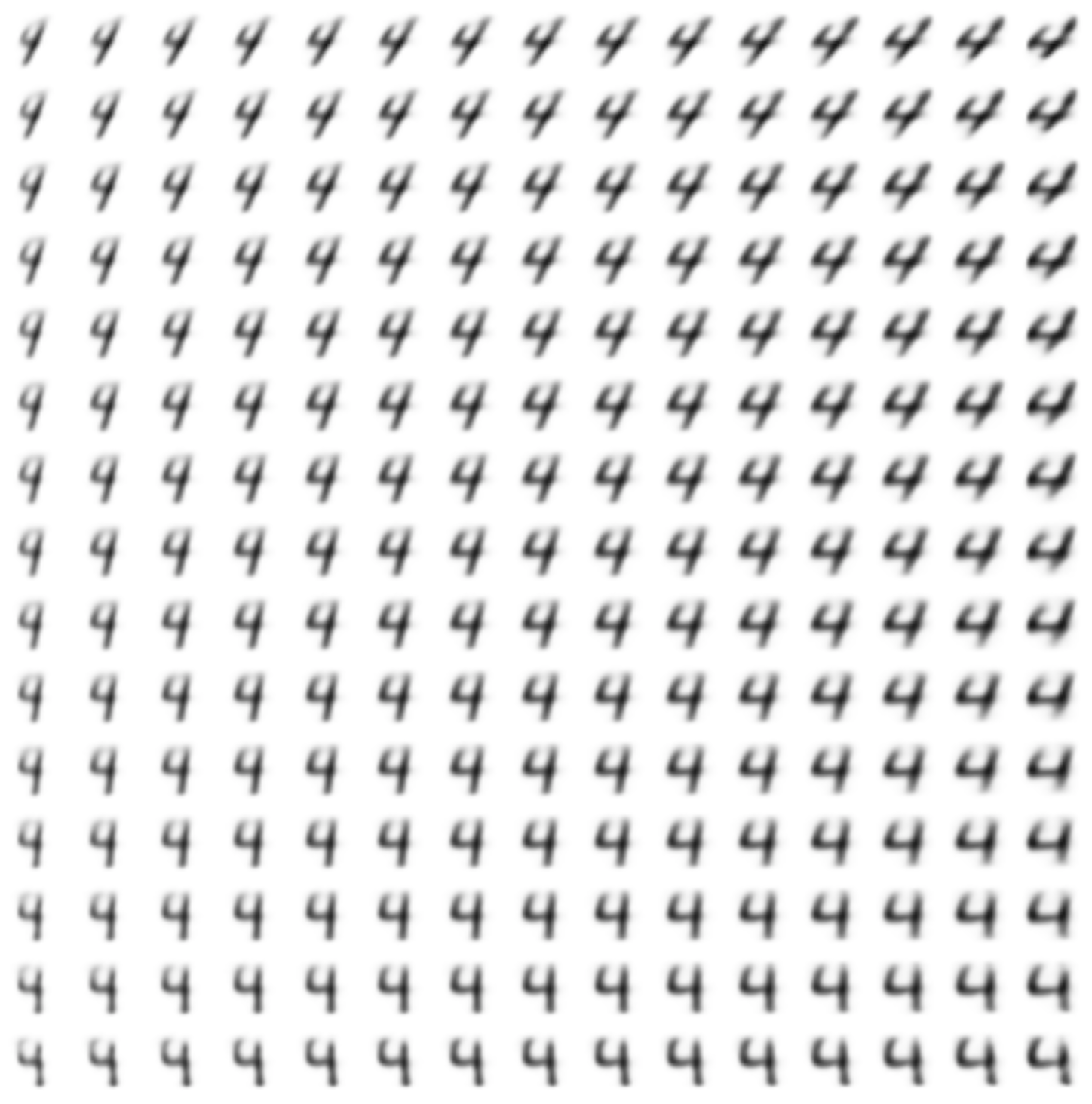
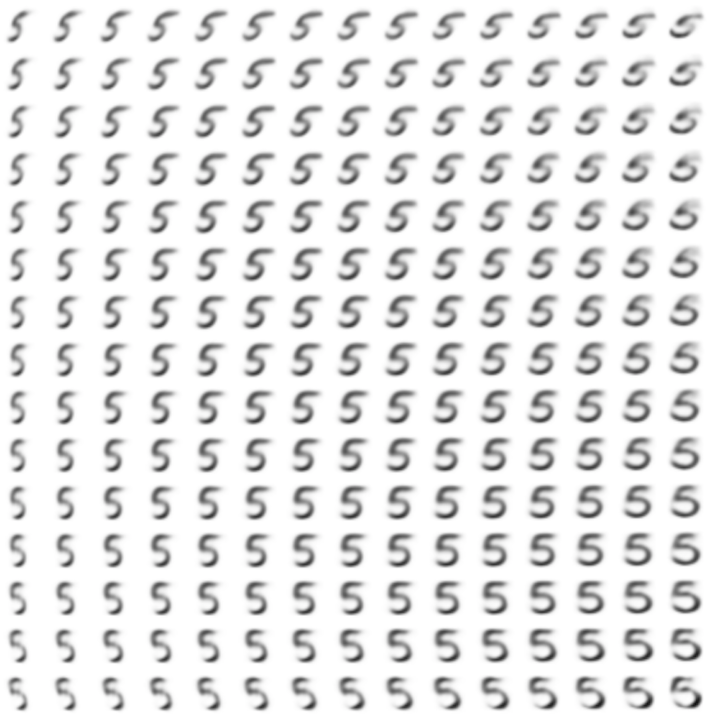
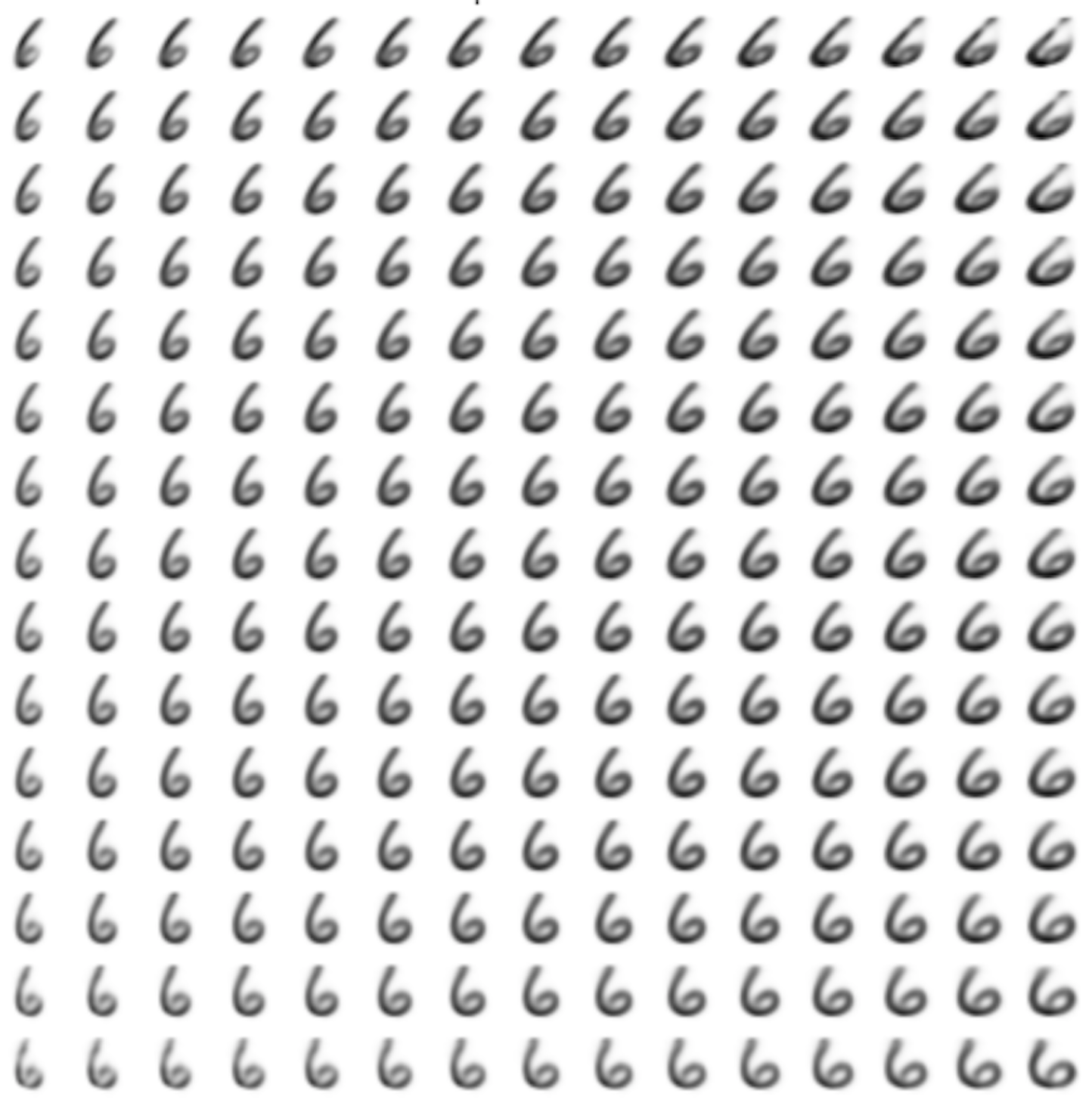
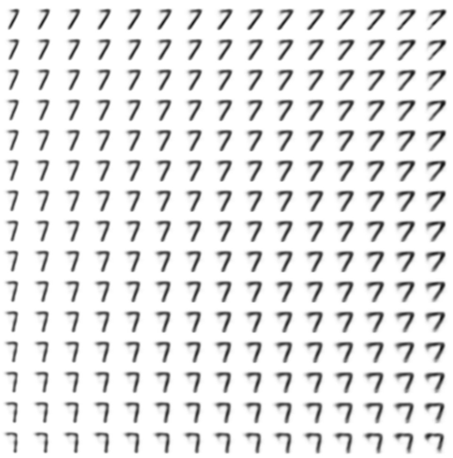
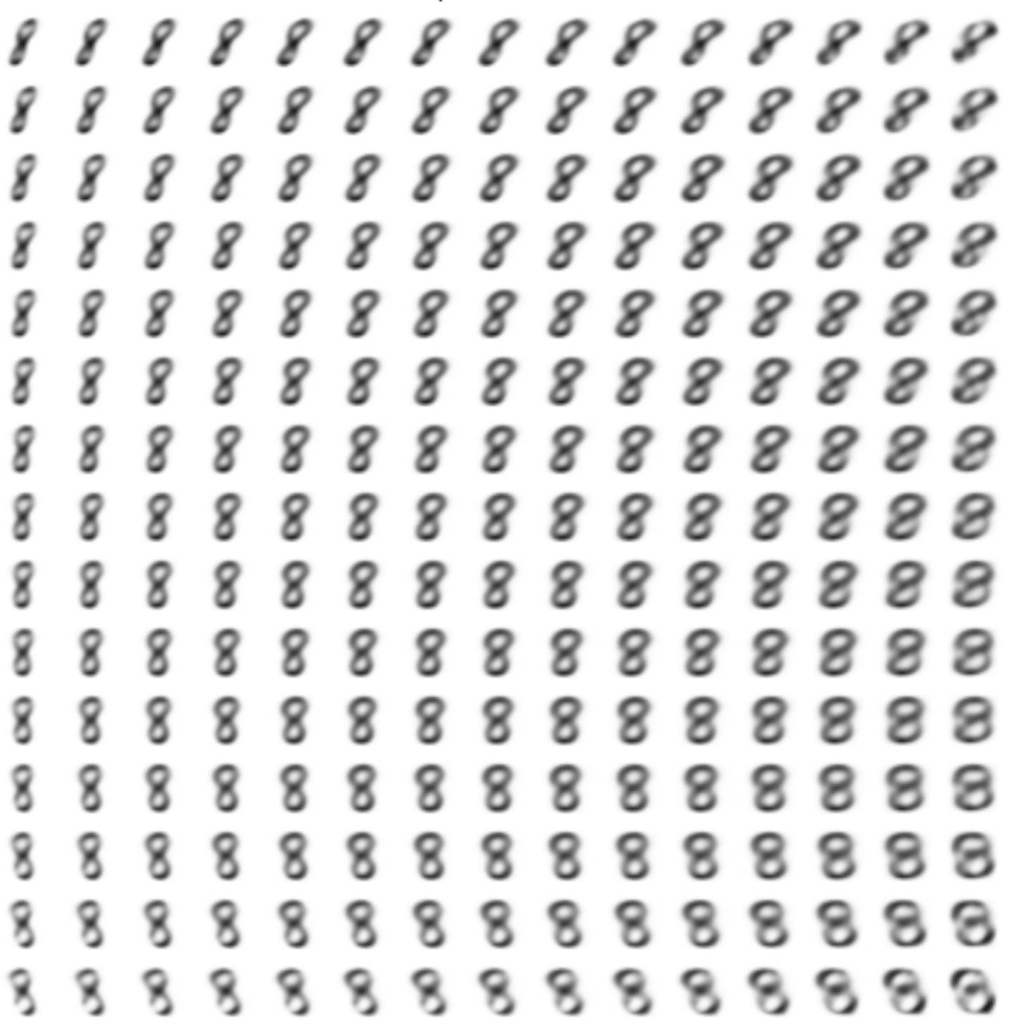
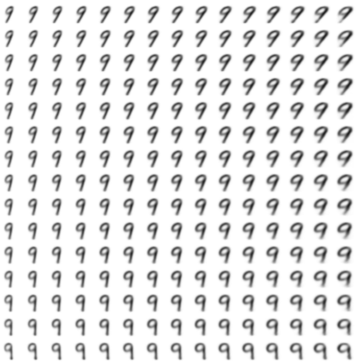
Generating numbers of a given label from and distribution for each label
Heavy gifs


Transferring the style of this model
As the sources of the style, we take the first ten "7" -ok, and based on their code
create the remaining numbers.Code
def style_transfer(model, X, lbl_in, lbl_out): rows = X.shape[0] if isinstance(lbl_in, int): lbl = lbl_in lbl_in = np.zeros((rows, 10)) lbl_in[:, lbl] = 1 if isinstance(lbl_out, int): lbl = lbl_out lbl_out = np.zeros((rows, 10)) lbl_out[:, lbl] = 1 return model.predict([X, lbl_in, lbl_out]) n = 10 lbl = 7 generated = [] prot = x_train[y_train == lbl][:n] for i in range(num_classes): generated.append(style_transfer(models["style_t"], prot, lbl, i)) generated[lbl] = prot plot_digits(*generated, invert_colors=True) The style has been transferred quite successfully: the slope and thickness of the stroke are preserved.
More style properties could be transferred simply by increasing the dimension.
It would also make the numbers less blurry.In the next part, we will look at how, using generative competing networks (GAN) , to generate numbers that are almost indistinguishable from the real ones, and after that, how to combine GANs with autoencoders.
GIF creation code
Code
from matplotlib.animation import FuncAnimation from matplotlib import cm import matplotlib def make_2d_figs_gif(figs, epochs, c, fname, fig): norm = matplotlib.colors.Normalize(vmin=0, vmax=1, clip=False) im = plt.imshow(np.zeros((28,28)), cmap='Greys', norm=norm) plt.grid(None) plt.title("Label: {}\nEpoch: {}".format(c, epochs[0])) def update(i): im.set_array(figs[i]) im.axes.set_title("Label: {}\nEpoch: {}".format(c, epochs[i])) im.axes.get_xaxis().set_visible(False) im.axes.get_yaxis().set_visible(False) return im anim = FuncAnimation(fig, update, frames=range(len(figs)), interval=100) anim.save(fname, dpi=80, writer='imagemagick') def make_2d_scatter_gif(zs, epochs, c, fname, fig): im = plt.scatter(zs[0][:, 0], zs[0][:, 1]) plt.title("Label: {}\nEpoch: {}".format(c, epochs[0])) def update(i): fig.clear() im = plt.scatter(zs[i][:, 0], zs[i][:, 1]) im.axes.set_title("Label: {}\nEpoch: {}".format(c, epochs[i])) im.axes.set_xlim(-5, 5) im.axes.set_ylim(-5, 5) return im anim = FuncAnimation(fig, update, frames=range(len(zs)), interval=100) anim.save(fname, dpi=80, writer='imagemagick') for lbl in range(num_classes): make_2d_figs_gif(figs[lbl], epochs, lbl, "./figs4/manifold_{}.gif".format(lbl), plt.figure(figsize=(7,7))) make_2d_scatter_gif(latent_distrs[lbl], epochs, lbl, "./figs4/z_distr_{}.gif".format(lbl), plt.figure(figsize=(7,7))) Useful links and literature
The theoretical part is based on the article:
[1] Tutorial on Variational Autoencoders, Carl Doersch, https://arxiv.org/abs/1606.05908
and in fact is its summary.
Many pictures are taken from Isaac Dykeman blog:
[2] Isaac Dykeman, http://ijdykeman.imtqy.com/ml/2016/12/21/cvae.html
Read more about the distance of Kullback-Leibler in Russian can be in
[3] http://www.machinelearning.ru/wiki/images/d/d0/BMMO11_6.pdf
The code is partly based on the Francois Chollet article:
[4] https://blog.keras.io/building-autoencoders-in-keras.html
Other interesting links:
http://blog.fastforwardlabs.com/2016/08/12/introducing-variational-autoencoders-in-prose-and.html
http://kvfrans.com/variational-autoencoders-explained/
Source: https://habr.com/ru/post/331664/
All Articles