Image smoothing by Peron and Malik anisotropic diffusion filter
The Peron and Malik anisotropic diffusion filter is a smoothing digital image filter, the key feature of which is that, while smoothing, it preserves and “enhances” the borders of the regions in the image.
In the article I will briefly consider why this filter is needed, the theory on it and how to implement it algorithmically, I will give the code in the Fortran language and examples of smoothed images.
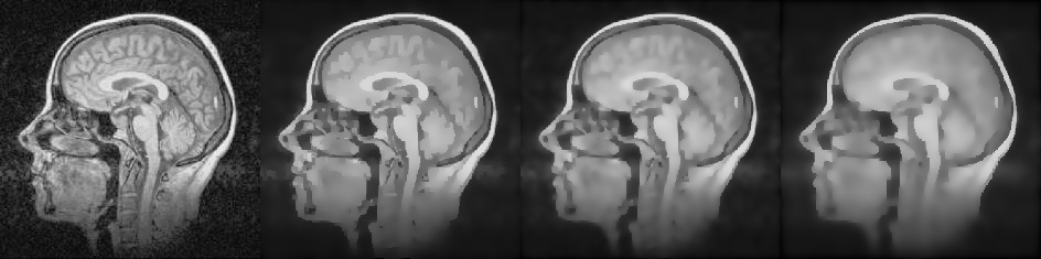
The leftmost image is original, to the right of the original - filtered with various parameters.
In image processing (especially in computer vision), segmentation problems or the demarcation of regions are often encountered. But if an image is obtained as a result of processing information from some physical device such as a camera, tomograph, etc., then it is usually noisy, and the nature of the noise in the image may be different, both due to physical phenomena and various algorithmic and hardware features.
')
Noises greatly complicate the tasks of segmentation and selection of borders, therefore, usually, such an image is first passed through some smoothing filters, which, in addition to smoothing noises, smooth everything else, which is good for the same segmentation, because there are fewer unimportant details. The image, if we consider it as a function of two variables, becomes smoother, which greatly facilitates the selection of areas on it.
However, when using such filters, we also smooth out the borders of the areas inside the image. That is, the stronger the smoothing, the more we move away from the original boundaries. In some tasks this may be acceptable, but, for example, in medicine, in automatic segmentation of tomography images of various parts of the human body, it is important to preserve the original boundaries of the regions (here, the internal organs, their deformations, various tumors, etc.) .
There is no formal mathematically strictly defining the boundary of a region for an arbitrary image (this would solve a lot of problems in image processing theory).
It was first described in the article by these mathematicians in 1990 (the link to the article is given in the “sources” at the end of the post). We will not go into deep theoretical details, but at least superficially consider how the filter works.
Hereinafter, images in grayscale are considered. For color, you can perform smoothing for each channel independently.
So, in the anisotropic diffusion filter, the smoothed image is some member of the family of images obtained by solving the following equation of mathematical physics:
With the initial condition:
Where:
- one-parameter family of images; the more the greater the degree of blur of the original image;
- the original image;
- derivative with respect to ;
- divergence operator;
- gradient;
From the point of view of theory, the image is a continuous function of two variables, and the picture itself (pixel matrix) is the discretization of this function. Moreover, 0 corresponds to zero brightness of the image point, that is, it indicates black color.
At its core, the anisotropic diffusion filter is a modification of the Gauss filter.
If we substitute the function not yet considered unit that is , then the isotropic diffusion equation is obtained:
Mathematicians Coderink and Gumel showed what a family of blurry images is by parameter , can be equivalently obtained as a solution of the convolution equation of the image function with the Gauss kernel (this is the Gauss filter):
Where:
- convolution operator;
- Gauss kernel function with zero expectation and standard deviation;
Obviously function plays the role of some "smoothing regulator".
Based on the filter equation ( 1 ), to maintain the original value at the point of the image, the time derivative should be zero (that is, the value on any blur layers would be constant). We get the following conditions on the function :
- at the borders;
- inside the regions, in other words, the usual Gaussian blur should occur inside the regions;
Perona and Malik used the gradient function of the image as simple to calculate and fairly accurate approximation of the boundaries of regions. The higher the gradient rate, the clearer the border. Based on this, we obtain:
Where - some function with a range of values on the segment .
Due to the fuzzy definition of boundaries through the norm of the gradient, the function is also required was monotonous diminishing.
Perona and Malik have proposed two options for the function. :
Where - a parameter determined either experimentally or by some “noise meter”.
Let us consider in more detail the second function (formula 3). To do this, build the graphs of the function for several different .
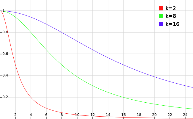
It can be seen that the more the greater the value of the function for any fixed point.
For example, at some point in the image, let's call it we know the value of the gradient rate at the level : . Then , while . It turns out in the first case, we weakly “smoothed out” the value at the point, since, according to the previously introduced criterion, it most likely lies on the border, and in the second, the value of the function practically one, respectively, the point is not considered boundary and will be smoothed out by the usual Gaussian blur.
In this way, acts as a "barrier" for noise, and with increasing the “requirement” that the point will be considered boundary increases.
In order to go directly to the filter algorithm, let's make a discretization of the equation. Quite simple in terms of mathematical calculations and undemanding to calculations will be the discretization of the equation by the method of finite differences. For convenience, we rewrite the basic equation:
Now we write the finite difference explicit scheme:
Writing the stability condition for the resulting explicit scheme is a non-trivial task due to the nonlinearity of the equation. But Perona and Malik determined that with the scheme will be sustainable for all . Given this fact and the fact that the discrete representation of the image function will be a matrix of pixel values, we will rewrite the main design scheme in the matrix form:
Where:
To calculate the coefficients first you need to calculate the rate of the gradient. The easiest way to approximate the gradient rate is to replace it with the length of the gradient projection on the corresponding axis of the difference grid.
Although this is a fairly crude replacement, approximating a slightly different diffusion equation, it nevertheless also preserves the overall image brightness and also gives almost identical results in comparison with a more accurate approximation of the gradient rate, winning the latter in computation speed.
The final calculation formula will look like this:
Where:
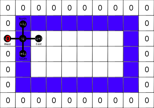
Schematically, the design scheme can be represented as in the figure below.
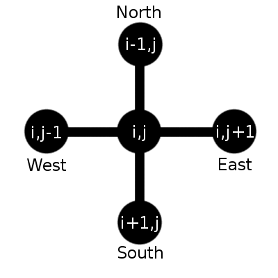
That is, the new value depends on the current value and the values of the four neighbors of the matrix cell. The question arises - how to recalculate the boundary cells, because the design scheme in this case will go beyond the matrix.
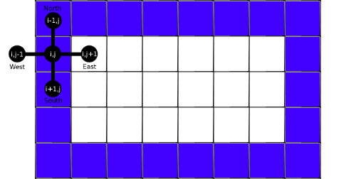
In order for the filter to change the brightness values in the cells within the maximum and minimum brightness of the original image, the process described by the basic equation must be adiabatic. From here we have the Dirichlet boundary condition of the form: . That is, just fill the border with zeros.
Based on the calculation formula, you will always have to keep at least two two-dimensional arrays in the memory, the first will correspond to the original image, the second will be blurred. If we draw an analogy with the Gauss filter, then to blur an image with a radius in the Peron and Malik filter we need to execute repetitions of the full recalculation of the image, each time replacing the image from the previous blur layer with the “original” one.
The sequence of actions will be something like this:
For color images, the principle of operation is preserved, but the recalculation must be performed for each channel separately.
In fact, the algorithm is quite trivial and can easily be programmed in many popular languages. I once faced with the difficulty of implementation on FORTRAN, because for a long time I could not find a good manual or a textbook on the language. Therefore, I want to give the implementation in this language, in the hope that it will be useful to someone.
Oddly enough, the main difficulty in programming was in reading the picture. In Fortran, there are no embedded procedures (in the language they are called “sub-rituals”) for manipulating images, but there is everything you need to implement your procedures.
The simplest format, which is also understood by many graphic editors, was PGM P5. This is an open format for storing bitmap bitmap images without compression in grayscale. It has a simple ASCII header, and the image itself is a sequence of single-byte (for shades of gray from 0 to 255) unsigned integers. More information about the format you can read directly in the standard itself, the link is given in the sources section.
I have designed the procedure for working with PGM as a module, I will not analyze it in detail, since this does not apply to the main topic, I will provide only a link to the source code . This module only works with images with a maximum gray value of 255.
We will start the program by connecting the module for working with PGM and declaring all the necessary variables.
The
Now consider the dimensions of the input image in the variables
Allocate memory for the image array and the array of the smoothed image and count the first data from the
Fortran allows the programmer to determine the index of the first element in the array himself, therefore, taking into account that there must be zeros around the image, we prefill the matrix u with zeros, setting its size from
The
Although in this case it does not matter, I want to note that the image will be read in transposed form, since Fortran stores two-dimensional arrays as a sequence of columns, and PGM format stores images as a sequence of rows.
We now turn to the most smoothing.
Everything is obvious here, the only thing that may not be entirely obvious to newbies in Fortran is the nesting of cycles, namely, the cycle in
At the end of the program, save the resulting smoothed image and free the memory.
The
It remains to define the function
→ Link to full program code
I compiled everything via gfortran with the following command (provided that all the files are in the same directory):
To begin with, let's compare the blur of the Peron and Malik filter with the Gaussian blur with
same
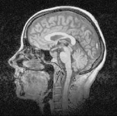
Source image
Smooth this image with a Gaussian filter and an anisotropic diffusion filter.
Consider another image.
Gaussian smoothing (
Filtering by Peron and Malik (

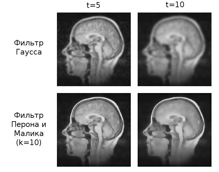
It is clearly seen as Gaussian blurring strongly smears the boundaries of the regions, while the anisotropic diffusion filter as a whole preserves them.
Let's experiment now with parameters. We will vary
Note that the boundaries of large areas do not shift with increasing
Let's see how the algorithm behaves for different time steps (
The images were almost identical. Now let's try to break the stability condition.
As we see, with small deviations some blur still occurs, but artifacts begin to appear. When
One of the possible approximations of the anisotropic diffusion filter was considered. In general, you can experiment with other functions. , enter the noise analysis function for automatic parameter selection .
In comparison with Gaussian blur, it can be seen that the filter really well preserves the borders of the regions. At the same time, the algorithm is rather expensive for calculations in comparison with the classical Gauss filter and cannot be well optimized either. Therefore, the Peron and Malik filter is mainly used in tasks where real-time operation is not required, but accuracy is more important.
I will reiterate references to source codes: a module for working with PGM , implementing a filter .
In the article I will briefly consider why this filter is needed, the theory on it and how to implement it algorithmically, I will give the code in the Fortran language and examples of smoothed images.
The leftmost image is original, to the right of the original - filtered with various parameters.
Introduction
In image processing (especially in computer vision), segmentation problems or the demarcation of regions are often encountered. But if an image is obtained as a result of processing information from some physical device such as a camera, tomograph, etc., then it is usually noisy, and the nature of the noise in the image may be different, both due to physical phenomena and various algorithmic and hardware features.
')
Noises greatly complicate the tasks of segmentation and selection of borders, therefore, usually, such an image is first passed through some smoothing filters, which, in addition to smoothing noises, smooth everything else, which is good for the same segmentation, because there are fewer unimportant details. The image, if we consider it as a function of two variables, becomes smoother, which greatly facilitates the selection of areas on it.
However, when using such filters, we also smooth out the borders of the areas inside the image. That is, the stronger the smoothing, the more we move away from the original boundaries. In some tasks this may be acceptable, but, for example, in medicine, in automatic segmentation of tomography images of various parts of the human body, it is important to preserve the original boundaries of the regions (here, the internal organs, their deformations, various tumors, etc.) .
There is no formal mathematically strictly defining the boundary of a region for an arbitrary image (this would solve a lot of problems in image processing theory).
Peron and Malik filter
It was first described in the article by these mathematicians in 1990 (the link to the article is given in the “sources” at the end of the post). We will not go into deep theoretical details, but at least superficially consider how the filter works.
Hereinafter, images in grayscale are considered. For color, you can perform smoothing for each channel independently.
Theory
So, in the anisotropic diffusion filter, the smoothed image is some member of the family of images obtained by solving the following equation of mathematical physics:
With the initial condition:
Where:
- one-parameter family of images; the more the greater the degree of blur of the original image;
- the original image;
- derivative with respect to ;
- divergence operator;
- gradient;
From the point of view of theory, the image is a continuous function of two variables, and the picture itself (pixel matrix) is the discretization of this function. Moreover, 0 corresponds to zero brightness of the image point, that is, it indicates black color.
At its core, the anisotropic diffusion filter is a modification of the Gauss filter.
If we substitute the function not yet considered unit that is , then the isotropic diffusion equation is obtained:
Mathematicians Coderink and Gumel showed what a family of blurry images is by parameter , can be equivalently obtained as a solution of the convolution equation of the image function with the Gauss kernel (this is the Gauss filter):
Where:
- convolution operator;
- Gauss kernel function with zero expectation and standard deviation;
Obviously function plays the role of some "smoothing regulator".
Based on the filter equation ( 1 ), to maintain the original value at the point of the image, the time derivative should be zero (that is, the value on any blur layers would be constant). We get the following conditions on the function :
- at the borders;
- inside the regions, in other words, the usual Gaussian blur should occur inside the regions;
Perona and Malik used the gradient function of the image as simple to calculate and fairly accurate approximation of the boundaries of regions. The higher the gradient rate, the clearer the border. Based on this, we obtain:
Where - some function with a range of values on the segment .
Due to the fuzzy definition of boundaries through the norm of the gradient, the function is also required was monotonous diminishing.
Perona and Malik have proposed two options for the function. :
Where - a parameter determined either experimentally or by some “noise meter”.
Let us consider in more detail the second function (formula 3). To do this, build the graphs of the function for several different .
It can be seen that the more the greater the value of the function for any fixed point.
For example, at some point in the image, let's call it we know the value of the gradient rate at the level : . Then , while . It turns out in the first case, we weakly “smoothed out” the value at the point, since, according to the previously introduced criterion, it most likely lies on the border, and in the second, the value of the function practically one, respectively, the point is not considered boundary and will be smoothed out by the usual Gaussian blur.
In this way, acts as a "barrier" for noise, and with increasing the “requirement” that the point will be considered boundary increases.
Sampling
In order to go directly to the filter algorithm, let's make a discretization of the equation. Quite simple in terms of mathematical calculations and undemanding to calculations will be the discretization of the equation by the method of finite differences. For convenience, we rewrite the basic equation:
Now we write the finite difference explicit scheme:
Writing the stability condition for the resulting explicit scheme is a non-trivial task due to the nonlinearity of the equation. But Perona and Malik determined that with the scheme will be sustainable for all . Given this fact and the fact that the discrete representation of the image function will be a matrix of pixel values, we will rewrite the main design scheme in the matrix form:
Where:
To calculate the coefficients first you need to calculate the rate of the gradient. The easiest way to approximate the gradient rate is to replace it with the length of the gradient projection on the corresponding axis of the difference grid.
Although this is a fairly crude replacement, approximating a slightly different diffusion equation, it nevertheless also preserves the overall image brightness and also gives almost identical results in comparison with a more accurate approximation of the gradient rate, winning the latter in computation speed.
The final calculation formula will look like this:
Where:
Schematically, the design scheme can be represented as in the figure below.
That is, the new value depends on the current value and the values of the four neighbors of the matrix cell. The question arises - how to recalculate the boundary cells, because the design scheme in this case will go beyond the matrix.
In order for the filter to change the brightness values in the cells within the maximum and minimum brightness of the original image, the process described by the basic equation must be adiabatic. From here we have the Dirichlet boundary condition of the form: . That is, just fill the border with zeros.
Algorithm and implementation in Fortran
Based on the calculation formula, you will always have to keep at least two two-dimensional arrays in the memory, the first will correspond to the original image, the second will be blurred. If we draw an analogy with the Gauss filter, then to blur an image with a radius in the Peron and Malik filter we need to execute repetitions of the full recalculation of the image, each time replacing the image from the previous blur layer with the “original” one.
The sequence of actions will be something like this:
- Determine the width and height of the image (let's call w and h, respectively);
- We allocate memory for a two-dimensional array of dimension (w + 2) * (h + 2) (let's call it I);
- We allocate memory for a two-dimensional array of dimension (w + 2) * (h + 2) (let's call BlurI);
- Fill the array with zeros I = 0;
- We read the image and write the pixel data to the center of the array I (that is, we leave one zero column or row left, right, above, below);
- Repeat until level <t (first level = 0);
- We recalculate all the cells of the array I using formula 4 , taking into account the offset indexing due to zero fields. Believe that - this is BlurI, but - I;
- Replace the image data in I with BlurI;
- Increment the counter, level = level + deltaT, where deltaT is a parameter, time step;
- Create and save an image from the data in the BlurI array. This is our blurred image;
- We release the memory, exit the program;
For color images, the principle of operation is preserved, but the recalculation must be performed for each channel separately.
Implementation on fortran
In fact, the algorithm is quite trivial and can easily be programmed in many popular languages. I once faced with the difficulty of implementation on FORTRAN, because for a long time I could not find a good manual or a textbook on the language. Therefore, I want to give the implementation in this language, in the hope that it will be useful to someone.
Oddly enough, the main difficulty in programming was in reading the picture. In Fortran, there are no embedded procedures (in the language they are called “sub-rituals”) for manipulating images, but there is everything you need to implement your procedures.
The simplest format, which is also understood by many graphic editors, was PGM P5. This is an open format for storing bitmap bitmap images without compression in grayscale. It has a simple ASCII header, and the image itself is a sequence of single-byte (for shades of gray from 0 to 255) unsigned integers. More information about the format you can read directly in the standard itself, the link is given in the sources section.
I have designed the procedure for working with PGM as a module, I will not analyze it in detail, since this does not apply to the main topic, I will provide only a link to the source code . This module only works with images with a maximum gray value of 255.
We will start the program by connecting the module for working with PGM and declaring all the necessary variables.
program blur use pgmio implicit none double precision, parameter :: t=10.0d0, deltaT=0.2d0, k=10.0d0 character*(*), parameter :: input='dif_tomography.pgm', output='output.pgm' double precision, allocatable :: u(:,:), nu(:,:) double precision :: north, south, east, west, level integer :: w, h, offset, n, i, j end program blur The
t parameter is the blur level at which we want to stop the algorithm, the deltaT is the time step, k is the parameter for the as yet not described function g . Input and output - the file with the original image and the output file, respectively.Now consider the dimensions of the input image in the variables
w and h . call pgmsize(input, w, h, offset) Offset determines the number of bytes allocated for the image header.Allocate memory for the image array and the array of the smoothed image and count the first data from the
input file. allocate(u(0:w+1,0:h+1)) u=0 allocate(nu(w,h)) call pgmread(input, offset, w, h, u, 0, 0) Fortran allows the programmer to determine the index of the first element in the array himself, therefore, taking into account that there must be zeros around the image, we prefill the matrix u with zeros, setting its size from
0 to w+1 for the first dimension, and from 0 to h+1 for the second . This will allow for further conversion to use natural indexing without bias.The
pgmread procedure reads w*h bytes, passing the offset bytes (occupied by the PGM header) into the u array. The last two parameters inform the procedure that the count in the matrix u starts from zero in each dimension.Although in this case it does not matter, I want to note that the image will be read in transposed form, since Fortran stores two-dimensional arrays as a sequence of columns, and PGM format stores images as a sequence of rows.
We now turn to the most smoothing.
level = 0 ! do while (level<t) do j=1,h do i=1,w north = u(i-1,j)-u(i,j) south = u(i+1,j)-u(i,j) east = u(i,j+1)-u(i,j) west = u(i,j-1)-u(i,j) nu(i,j) = u(i,j) + deltaT*(g(north)*north+g(south)*south+g(east)*east+g(west)*west) end do end do u(1:w,1:h) = nu(1:w,1:h) ! level = level + deltaT end do Everything is obvious here, the only thing that may not be entirely obvious to newbies in Fortran is the nesting of cycles, namely, the cycle in
j comes before the cycle in i . All, again, due to the fact that Fortran stores two-dimensional arrays in memory as a sequence of columns. If we place loops in places, the program will also work, but much slower - the program will not bypass the memory sequentially, but will run from different cells to and fro.At the end of the program, save the resulting smoothed image and free the memory.
deallocate(u) call pgmwriteheader(output, w, h) call pgmappendbytes(output, nu, 1, 1) deallocate(nu) The
pgmwriteheader procedure creates an output file and writes a PGM P5 header to it. The pgmappendbytes procedure writes a sequence of bytes from nu to the end of the output file, given that nu indices start with 1 in both dimensions. I note that pgmappendbytes writes bytes from a two-dimensional array, again in the order of the columns, therefore, although there was a transposed version of the image in memory, the image was transposed back when recording.It remains to define the function
g . For example, we implement the function according to the formula 3 . contains function g(x) result(v) implicit none double precision, intent(in) :: x double precision :: v v = 1/(1+(x/k)**2) end function g → Link to full program code
I compiled everything via gfortran with the following command (provided that all the files are in the same directory):
gfortran pgmio.f90 blur.f90 Filter examples
To begin with, let's compare the blur of the Peron and Malik filter with the Gaussian blur with
same
t .Source image
Smooth this image with a Gaussian filter and an anisotropic diffusion filter.
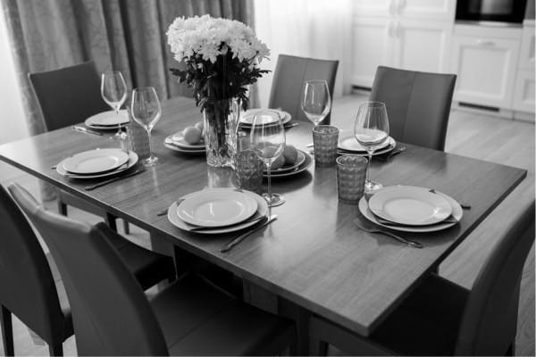
Consider another image.
Gaussian smoothing (
t=10 ).Filtering by Peron and Malik (
t=10, k=8 ).It is clearly seen as Gaussian blurring strongly smears the boundaries of the regions, while the anisotropic diffusion filter as a whole preserves them.
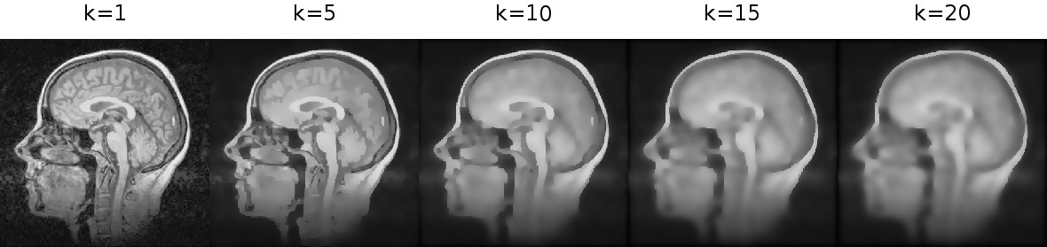
Let's experiment now with parameters. We will vary
k for the same t and deltaT ( t=10, deltaT=0.2 ).Note that the boundaries of large areas do not shift with increasing
k . But smaller areas gradually begin to merge. For a sufficiently large k, we actually obtain a Gaussian blur, since no point passes the condition on the boundary.Let's see how the algorithm behaves for different time steps (
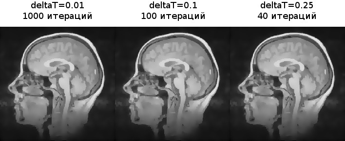
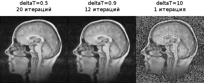
t=10,k=5 ).The images were almost identical. Now let's try to break the stability condition.
As we see, with small deviations some blur still occurs, but artifacts begin to appear. When
deltaT=10 they already fill the entire image.Conclusion
One of the possible approximations of the anisotropic diffusion filter was considered. In general, you can experiment with other functions. , enter the noise analysis function for automatic parameter selection .
In comparison with Gaussian blur, it can be seen that the filter really well preserves the borders of the regions. At the same time, the algorithm is rather expensive for calculations in comparison with the classical Gauss filter and cannot be well optimized either. Therefore, the Peron and Malik filter is mainly used in tasks where real-time operation is not required, but accuracy is more important.
I will reiterate references to source codes: a module for working with PGM , implementing a filter .
Sources
Source: https://habr.com/ru/post/331618/
All Articles