Selection of the distribution law of a random variable according to statistical sampling using Python tools
What can "tell" the laws of the distribution of random variables, if you learn how to "listen"
The laws of the distribution of random variables are the most "eloquent" in the statistical processing of measurement results. Adequate assessment of measurement results is possible only when the rules governing the behavior of measurement errors are known. The basis of these rules and constitute the laws of the distribution of errors, which can be represented in differential (pdf) or integral (cdf) forms.
The main characteristics of the laws of distribution include: the most probable value of the measured quantity called the expectation (mean) ; a measure of the dispersion of a random variable around the expectation called the standard deviation (std) .
Additional characteristics are - a measure of the crowding of the differential form of the distribution law about the axis of symmetry called asymmetry (skew) and a measure of coolness, the envelope of the differential form called excess (kurt) . The reader has already guessed that these abbreviations are taken from the scipy libraries. stats, numpy, which we will use.
The story about the laws of measurement error distribution would be incomplete, if not to mention the relationship between the entropy and root-mean-square value of the error. Without tiring readers with long calculations from the information theory of measurements [1], I will immediately formulate the result.
')
From the point of view of information, a normal distribution results in exactly the same amount of information as a uniform one. We write the expression for the error delta0 using the functions of the above libraries for the distribution of the random variable x .
This allows replacing any law of error distribution with a uniform one with the same value delta0 .
We introduce one more indicator - the entropy coefficient k, which for a normal distribution is equal to:
It should be noted that any distribution other than normal will have a lower entropy coefficient.
It is better to see once than seven times to read. For further comparative analysis of integral distributions: uniform, normal and logistic, we modernize the examples given in the documentation [2].
Program for normal distribution:
from scipy.stats import norm import matplotlib.pyplot as plt import numpy as np fig, ax = plt.subplots(1, 1) # Calculate a few first moments: mean, var, skew, kurt = norm.stats(moments='mvsk') # Display the probability density function (``pdf``): x = np.linspace(norm.ppf(0.01), norm.ppf(0.99), 100) ax.plot(x, norm.pdf(x), 'r-', lw=5, alpha=0.6, label='norm pdf') ax.plot(x, norm.cdf(x), 'b-', lw=5, alpha=0.6, label='norm cdf') # Check accuracy of ``cdf`` and ``ppf``: vals = norm.ppf([0.001, 0.5, 0.999]) np.allclose([0.001, 0.5, 0.999], norm.cdf(vals)) # True # Generate random numbers: r = norm.rvs(size=1000) # And compare the histogram: ax.hist(r, normed=True, histtype='stepfilled', alpha=0.2) ax.legend(loc='best', frameon=False) plt.show() 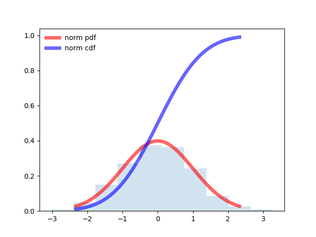
Program for even distribution:
from scipy.stats import uniform import matplotlib.pyplot as plt import numpy as np fig, ax = plt.subplots(1, 1) # Calculate a few first moments: #mean, var, skew, kurt = uniform.stats(moments='mvsk') # Display the probability density function (``pdf``): x = np.linspace(uniform.ppf(0.01), uniform.ppf(0.99), 100) ax.plot(x, uniform.pdf(x),'r-', lw=5, alpha=0.6, label='uniform pdf') ax.plot(x, uniform.cdf(x),'b-', lw=5, alpha=0.6, label='uniform cdf') # Check accuracy of ``cdf`` and ``ppf``: vals = uniform.ppf([0.001, 0.5, 0.999]) np.allclose([0.001, 0.5, 0.999], uniform.cdf(vals)) # True # Generate random numbers: r = uniform.rvs(size=1000) # And compare the histogram: ax.hist(r, normed=True, histtype='stepfilled', alpha=0.2) ax.legend(loc='best', frameon=False) plt.show() 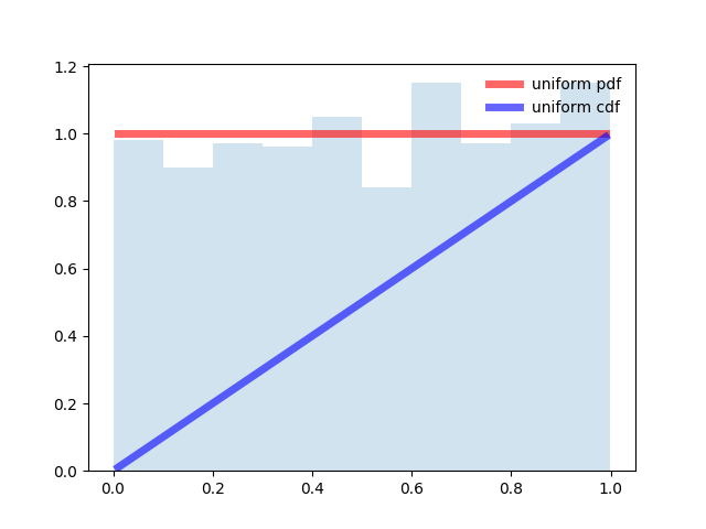
Program for logistic distribution.
from scipy.stats import logistic import matplotlib.pyplot as plt import numpy as np fig, ax = plt.subplots(1, 1) # Calculate a few first moments: mean, var, skew, kurt = logistic.stats(moments='mvsk') # Display the probability density function (``pdf``): x = np.linspace(logistic.ppf(0.01), logistic.ppf(0.99), 100) ax.plot(x, logistic.pdf(x), 'g-', lw=5, alpha=0.6, label='logistic pdf') ax.plot(x, logistic.cdf(x), 'r-', lw=5, alpha=0.6, label='logistic cdf') vals = logistic.ppf([0.001, 0.5, 0.999]) np.allclose([0.001, 0.5, 0.999], logistic.cdf(vals)) # True # Generate random numbers: r = logistic.rvs(size=1000) # And compare the histogram: ax.hist(r, normed=True, histtype='stepfilled', alpha=0.2) ax.legend(loc='best', frameon=False) plt.show() 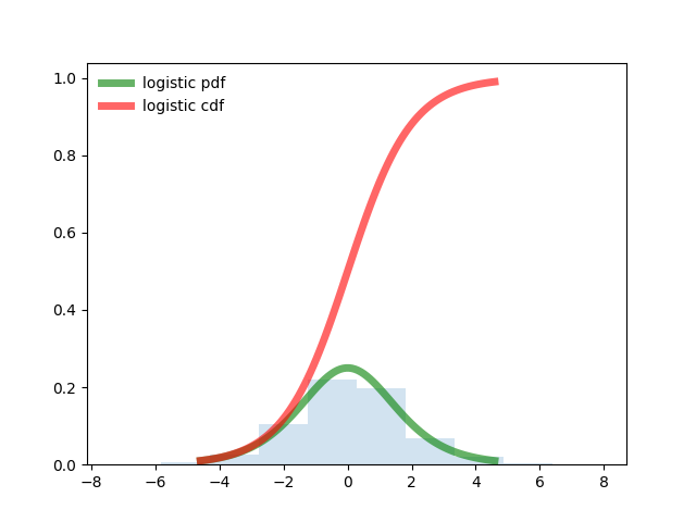
Now we know what the integral forms of the normal, uniform, and logistic laws look like and can proceed to their comparison with the test distribution, raising a more general question - the selection of the distribution law of a random variable according to the statistical sampling data.
How to choose the distribution law, having the integral probability distribution of the test sample
We will prepare the first part of the program, which will compare the listed integral distributions with the test sample. To do this, we define the basic parameters common for the laws of distribution — expectation and standard deviation, using a uniform distribution.
The first part of the program is designed to prepare for the comparison of the three laws of distribution in integral form.
from scipy.stats import logistic,uniform,norm,pearsonr from numpy import sqrt,pi,e import numpy as np import matplotlib.pyplot as plt fig, ax = plt.subplots(1, 1) n=1000# x=uniform.rvs(loc=0, scale=150, size=n)# x.sort()# print(" ( ) -%s"%str(round(np.mean(x),3))) print(" ( ) -%s"%str(round(np.std(x),3))) print(" -%s"%str(round(np.std(x)*sqrt(np.pi*np.e*0.5),3))) pu=uniform.cdf(x/(np.max(x)))# ax.plot(x,pu, lw=5, alpha=0.6, label='uniform cdf') pn=norm.cdf(x, np.mean(x), np.std(x))# ax.plot(x,pn, lw=5, alpha=0.6, label='norm cdf') pl=logistic.cdf(x, np.mean(x), np.std(x))# ax.plot(x,pl, lw=5, alpha=0.6, label='logistic cdf') Hereinafter, the results for comparison are entered into the print function to monitor the progress of the calculations.
The test integral distribution and the results of the comparison are given in the second part of the program. It determines the correlation coefficients between the test and each of the three integral distribution laws.
Since the correlation coefficients may differ slightly, an additional definition of the declared squares of deviation is introduced.
Second part of the program
p=np.arange(0,n,1)/n ax.plot(x,p, lw=5, alpha=0.6, label='test') ax.legend(loc='best', frameon=False) plt.show() print(" - %s"%str(round(pearsonr(pn,p)[0],3))) print(" - %s"%str(round(pearsonr(pl,p)[0],3))) print(" - %s"%str(round(pearsonr(pu,p)[0],3))) print(' -%i'%round(n*sum(((pn-p)/pn)**2))) print(' -%i'%round(n*sum(((pl-p)/pl)**2))) print(' -%i'%round(n*sum(((pu-p)/pu)**2))) The test function of the integral form of the distribution law is constructed in the form of step accumulation –0+ 1 / n + 2 / n + …… + 1
Schedule and result robots program.
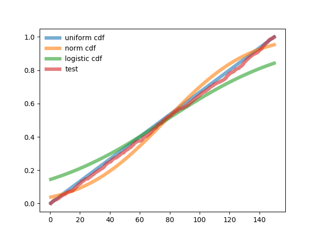
Mathematical expectation for the sample (total for compared distributions) - 77.3
MSE by sample (common for compared distributions) - 43.318
The entropy value of the error is 89.511
Correlation between normal distribution and test distribution - 0.994
Correlation between logistic distribution and test distribution - 0.998
The correlation between uniform distribution and test - 1.0
The weighted sum of squares of the deviation of the normal distribution from the test is 37082
Weighted sum of squares of deviation of the logistic distribution from the test - 75458
The weighted sum of the squares of the deviation of the uniform distribution from the test is 6622
The test probability distribution in integral form is uniform. With minimal differences in the correlation coefficient for a uniform distribution, the weighted deviation from the test one is 5.6 times less than that of the normal one and 11 times less than that of the logistic one.
Conclusion
The implementation of the selection of the distribution law of a random variable according to the statistical sampling may be useful in solving similar problems.
1. Elements of the information theory of measurement.
2. Statistical functions.
Source: https://habr.com/ru/post/331560/
All Articles