Content

• Part 1: Introduction
  
• Part 2: Manifold learning and latent variables
  
• Part 3: Variational autoencoders ( VAE )
  
• Part 4: Conditional VAE
  
• Part 5: GAN (Generative Adversarial Networks) and tensorflow
  
• Part 6: VAE + GAN
  

In the last part, we have already discussed what hidden variables are, looked at their distribution, and also understood that it is difficult to generate new objects from the distribution of hidden variables in ordinary autoencoders. In order to be able to generate new objects, the space of hidden variables ( latent variables ) must be predictable.

Variational Autoencoders ( Variational Autoencoders ) are autoencoders that learn to map objects into a given hidden space and, therefore, sample them. Therefore, variational autoencoders are also referred to the family of generative models.



Illustration of [2]
')
Having any one distribution can get any other for example, let - normal normal distribution, - also random distribution, but it looks completely different




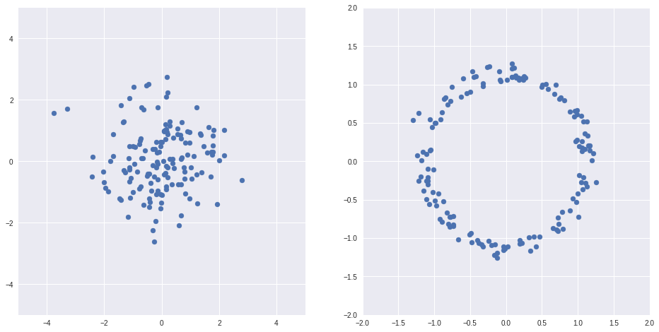
Example above from [1]

Thus, if you select the right functions, you can map the hidden variable spaces of regular autoencoders into some good spaces, for example, those where the distribution is normal. And then back.

On the other hand, it is not necessary to specifically study how to display some hidden spaces in others. If there are any useful hidden spaces, then the correct autoencoder will learn them along the way itself, but ultimately it will display the space we need.

---

Below is a challenging, but necessary theory underlying the VAE . I tried to squeeze out [1, Tutorial on Variational Autoencoders, Carl Doersch, 2016] all the most important things, dwelling in more detail on those places that seemed difficult for me.

Let be - hidden variables, and - data. Using the example of drawn numbers, consider the natural generative process that generated our sample:

• probability distribution of images of figures in the pictures, i.e. the probability of a particular image of a digit is in principle to be drawn (if the picture is not like a digit, then this probability is extremely small, and vice versa),
  
• - the probability distribution of hidden factors, for example, the distribution of the thickness of the stroke,
  
• - the probability distribution of pictures for given hidden factors, the same factors can lead to different pictures (the same person in the same conditions does not draw absolutely identical numbers).
  

Imagine as the sum of some generating function and some complicated noise


We want to build some artificial generative process that will create objects that are close in some metric to training .


and again


- some family of functions that our model represents, and - its parameters. Choosing a metric, we choose what kind of noise seems to us. . If metric then we consider the noise as normal and then:


According to the maximum likelihood principle, it remains for us to optimize the parameters in order to maximize i.e. the likelihood of objects from the sample.

The problem is that we cannot directly optimize the integral (1) directly: the space can be high-dimensional, there are many objects, and the metric is bad. On the other hand, if you think about it, then to each specific can only result in a very small subset for the rest will be very close to zero.
And with optimization it is enough to sample only good ones. .

In order to know which we need to sample, we introduce a new distribution which depending on will show the distribution which could lead to this .

We first write the Kullback-Leibler distance (an asymmetric measure of the "similarity" of two distributions, for more details [3] ) between
and real :


We apply the Bayes formula:


Select another Kullback-Leibler distance:


As a result, we obtain the identity:

---

---

This identity is the cornerstone of variational autoencoders , it is true for any and .

Let be and depend on parameters: and , but - normal then we get:


Let's take a closer look at what we did:

• First of all, , Suspiciously similar to the encoder and decoder (more precisely, the decoder is in terms of ),
  
• on the left in the identity - the value that we want to maximize for the elements of our training sample + some mistake which hopefully with enough capacity will go to 0,
  
• to the right is a value that we can optimize by gradient descent, where the first term has a sense of prediction quality decoder by values and the second term is the distance K-L between the distribution which the encoder predicts for a specific and distribution for all right away
  

In order to be able to optimize the right side of the gradient descent, it remains to deal with two things:

1. More precisely, we define what

Usually is selected by the normal distribution:


That is, an encoder for each predicts 2 values: average and variation normal distribution from which values ​​are already sampled. It all works like this:



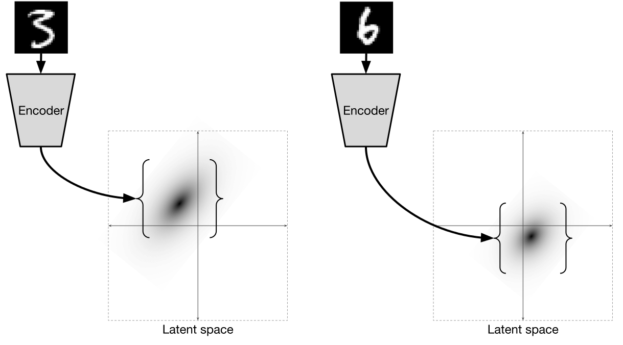
Illustration of [2]

Given that for each individual data point the encoder predicts some normal distribution


for marginal distribution : that comes from the formula, and it's awesome.



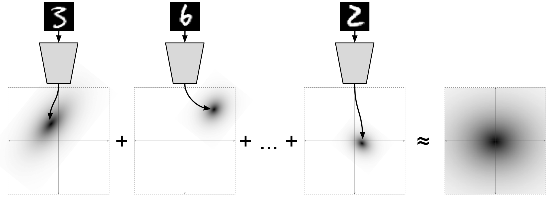
Illustration of [2]

Wherein takes the form:

2. We will understand how to distribute errors through

The fact is that here we take random values and pass them to the decoder.
It is clear that it is impossible to directly propagate errors through random values, so the so-called reparametrization trick is used .

The scheme is as follows:


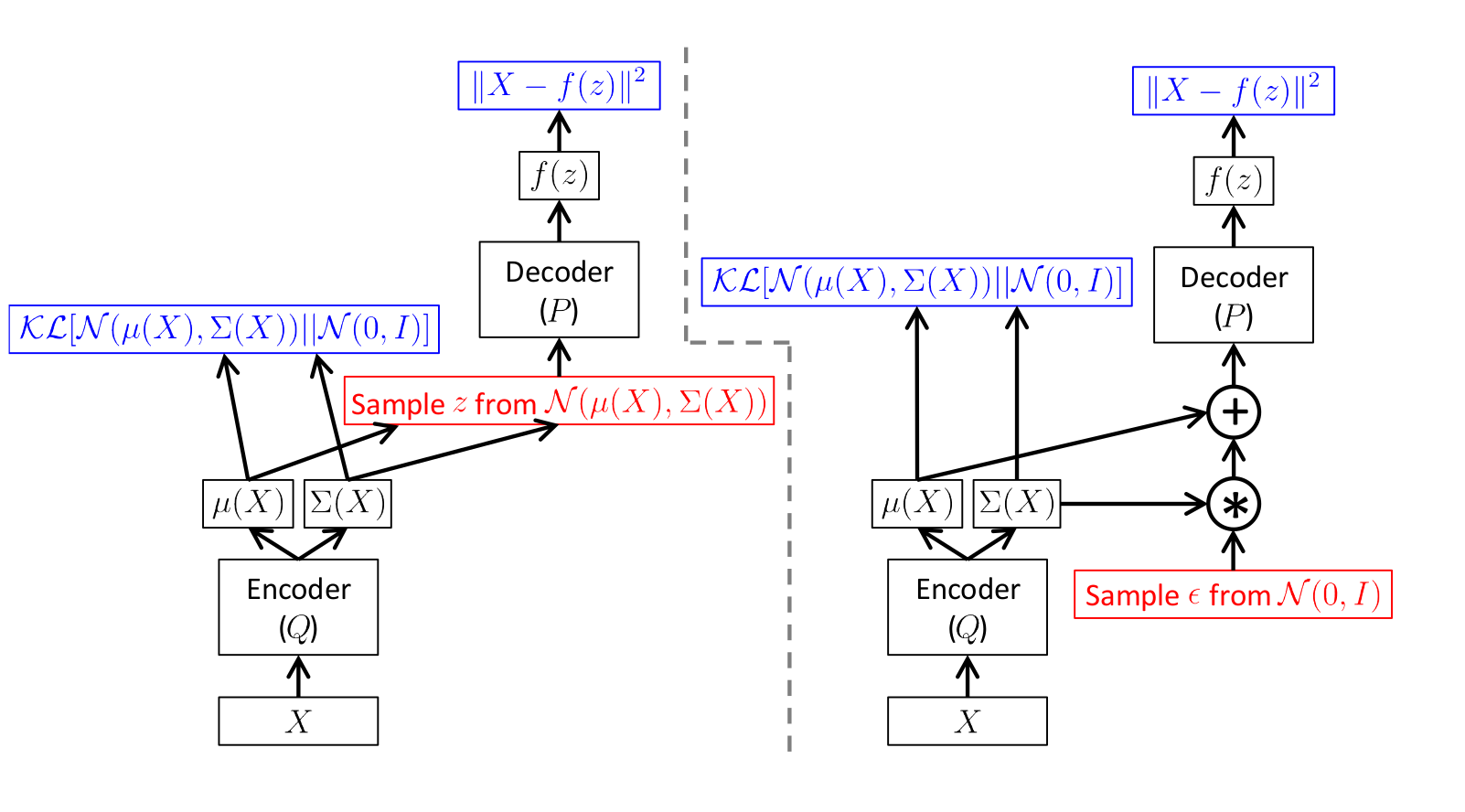
Illustration of [1]

Here on the left picture is a diagram without a trick, and on the right with a trick.
Sampling is shown in red, and error calculation in blue.
That is, in fact, just take the standard deviation predicted by the encoder. multiply by a random number of and add the predicted average .
The direct propagation on both schemes is absolutely the same, but on the right scheme the reverse error propagation works.

After we have trained such a variational autoencoder, the decoder becomes a full-fledged generative model. In essence, an encoder is needed mainly in order to train the decoder to be separately a generative model.


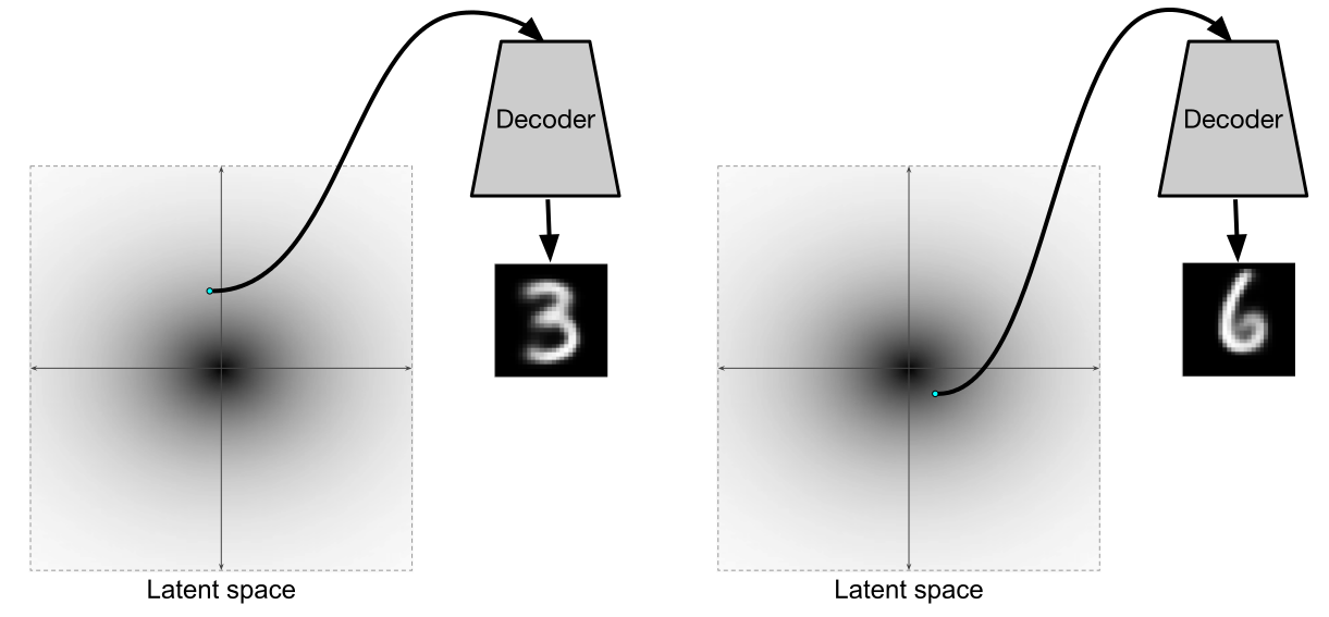
Illustration of [2]

Illustration of [1]

But the fact that the encoder and decoder instead form a full-fledged autoencoder is a very nice plus.

VAE in Keras

Now, when we figured out what variational autoencoders are, let's write one on Keras .

We import the necessary libraries and datasets:

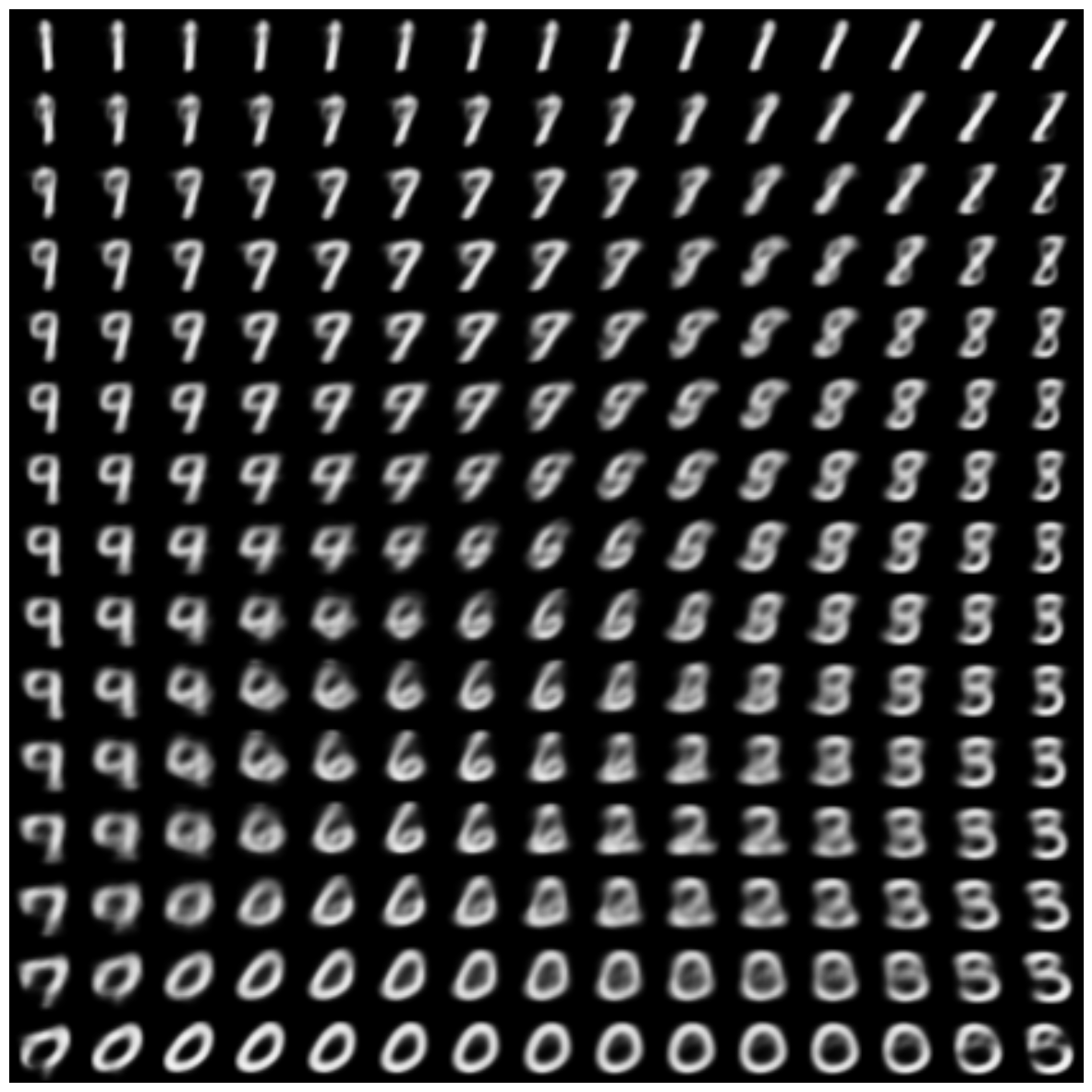
 import sys import numpy as np import matplotlib.pyplot as plt %matplotlib inline import seaborn as sns from keras.datasets import mnist (x_train, y_train), (x_test, y_test) = mnist.load_data() x_train = x_train.astype('float32') / 255. x_test = x_test .astype('float32') / 255. x_train = np.reshape(x_train, (len(x_train), 28, 28, 1)) x_test = np.reshape(x_test, (len(x_test), 28, 28, 1)) 

Let's set the main parameters. Hidden space will take dimension 2 to later generate from it and visualize the result.
Note : dimension 2 is extremely small, so you should expect that the numbers will be very blurry.

 batch_size = 500 latent_dim = 2 dropout_rate = 0.3 start_lr = 0.0001 

Let's write models of variational autoencoder.

In order for learning to occur faster and better, add dropout layers and batch normalization .

And in the decoder we use leaky ReLU as an activation, which we add as a separate layer after dense layers without activation.
The sampling function implements the sampling of values. of using the trick of reparameterization.

vae_loss is the right side of the equation:
will continue to be used as a loss.

 from keras.layers import Input, Dense from keras.layers import BatchNormalization, Dropout, Flatten, Reshape, Lambda from keras.models import Model from keras.objectives import binary_crossentropy from keras.layers.advanced_activations import LeakyReLU from keras import backend as K def create_vae(): models = {} #  Dropout  BatchNormalization def apply_bn_and_dropout(x): return Dropout(dropout_rate)(BatchNormalization()(x)) #  input_img = Input(batch_shape=(batch_size, 28, 28, 1)) x = Flatten()(input_img) x = Dense(256, activation='relu')(x) x = apply_bn_and_dropout(x) x = Dense(128, activation='relu')(x) x = apply_bn_and_dropout(x) #    #  ,    ,    z_mean = Dense(latent_dim)(x) z_log_var = Dense(latent_dim)(x) #   Q    def sampling(args): z_mean, z_log_var = args epsilon = K.random_normal(shape=(batch_size, latent_dim), mean=0., stddev=1.0) return z_mean + K.exp(z_log_var / 2) * epsilon l = Lambda(sampling, output_shape=(latent_dim,))([z_mean, z_log_var]) models["encoder"] = Model(input_img, l, 'Encoder') models["z_meaner"] = Model(input_img, z_mean, 'Enc_z_mean') models["z_lvarer"] = Model(input_img, z_log_var, 'Enc_z_log_var') #  z = Input(shape=(latent_dim, )) x = Dense(128)(z) x = LeakyReLU()(x) x = apply_bn_and_dropout(x) x = Dense(256)(x) x = LeakyReLU()(x) x = apply_bn_and_dropout(x) x = Dense(28*28, activation='sigmoid')(x) decoded = Reshape((28, 28, 1))(x) models["decoder"] = Model(z, decoded, name='Decoder') models["vae"] = Model(input_img, models["decoder"](models["encoder"](input_img)), name="VAE") def vae_loss(x, decoded): x = K.reshape(x, shape=(batch_size, 28*28)) decoded = K.reshape(decoded, shape=(batch_size, 28*28)) xent_loss = 28*28*binary_crossentropy(x, decoded) kl_loss = -0.5 * K.sum(1 + z_log_var - K.square(z_mean) - K.exp(z_log_var), axis=-1) return (xent_loss + kl_loss)/2/28/28 return models, vae_loss models, vae_loss = create_vae() vae = models["vae"] 

Note : we used a lambda layer with a function that samples from from the underlying framework, which clearly requires the size of the batch. In all models in which this layer is present, we are now forced to transfer just such a size of the batch (that is, in the encoder and vae ).

The optimization function will take Adam or RMSprop , both show good results.

 from keras.optimizers import Adam, RMSprop vae.compile(optimizer=Adam(start_lr), loss=vae_loss) 

Code for drawing rows of numbers and digits from a manifold


Often, in the process of learning the model, it is required to perform some actions: change the learning_rate , save intermediate results, save the model, draw pictures, etc.

To do this, keras have callbacks that are passed to the fit method before starting the training. For example, to influence the learning rate in the learning process, there are callbacks such as LearningRateScheduler , ReduceLROnPlateau , to save the model - ModelCheckpoint .

A separate callback is needed in order to follow the learning process in TensorBoard . It will automatically add to the log file all metrics and losses that are considered between eras.

For the case when arbitrary functions are required to be performed in the learning process, there is a LambdaCallback . It starts the execution of arbitrary functions at specified moments of training, for example, between eras or batch.
We will follow the learning process by studying how numbers are generated from .

 from IPython.display import clear_output from keras.callbacks import LambdaCallback, ReduceLROnPlateau, TensorBoard # ,     ,    figs = [] latent_distrs = [] epochs = [] # ,     save_epochs = set(list((np.arange(0, 59)**1.701).astype(np.int)) + list(range(10))) #       imgs = x_test[:batch_size] n_compare = 10 #  generator = models["decoder"] encoder_mean = models["z_meaner"] # ,       def on_epoch_end(epoch, logs): if epoch in save_epochs: clear_output() #   output #      decoded = vae.predict(imgs, batch_size=batch_size) plot_digits(imgs[:n_compare], decoded[:n_compare]) #   figure = draw_manifold(generator, show=True) #     z     epochs.append(epoch) figs.append(figure) latent_distrs.append(encoder_mean.predict(x_test, batch_size)) #  pltfig = LambdaCallback(on_epoch_end=on_epoch_end) # lr_red = ReduceLROnPlateau(factor=0.1, patience=25) tb = TensorBoard(log_dir='./logs') #   vae.fit(x_train, x_train, shuffle=True, epochs=1000, batch_size=batch_size, validation_data=(x_test, x_test), callbacks=[pltfig, tb], verbose=1) 

Now, if TensorBoard is installed, you can follow the learning process.

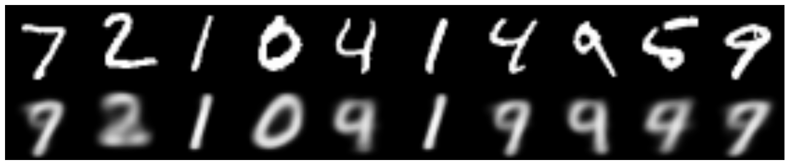
Here is how this encoder recovers images:



And here is the result of sampling from



Here is the process of learning how to generate numbers:


Distribution of codes in hidden space:


Not ideally normal, but rather close (especially, considering that the dimension of the hidden space is only 2).

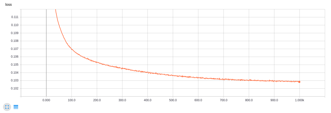
TensorBoard learning curve



It can be seen that dimension 2 for such a task is very small, the numbers are very blurry, and also in the intervals between good many ragged numbers.
In the next part, we will look at how to generate the numbers of the desired label, get rid of the ragged ones, and also how to transfer the style from one number to another.

Useful links and literature

The theoretical part is based on the article:
[1] Tutorial on Variational Autoencoders, Carl Doersch, 2016, https://arxiv.org/abs/1606.05908
and in fact is her summary

Many pictures are taken from Isaac Dykeman blog:
[2] Isaac Dykeman, http://ijdykeman.imtqy.com/ml/2016/12/21/cvae.html

You can read more about Kullback-Leibler distance in Russian here:
[3] http://www.machinelearning.ru/wiki/images/d/d0/BMMO11_6.pdf

The code is partly based on the Francois Chollet article:
[4] https://blog.keras.io/building-autoencoders-in-keras.html

Other interesting links:
http://blog.fastforwardlabs.com/2016/08/12/introducing-variational-autoencoders-in-prose-and.html
http://kvfrans.com/variational-autoencoders-explained/