Making data science portfolio: history through data
Translation suddenly successfully hit the stream of other datascript tutorials on Habré. :)
This one is written by Vic Paruchuri, the founder of Dataquest.io , where they are engaged in this kind of interactive training in data science and preparation for real work in this area. Some exclusive know-how is not here, but the process from data collection to initial conclusions about them is described in detail, which may be interesting not only for those who want to write a summary of data science, but also for those who just want to try their hand at practical analysis, but does not know where to start.
Data science companies are increasingly looking at their portfolios when they make decisions about hiring. This, in particular, due to the fact that the best way to judge practical skills is a portfolio. And the good news is that it is completely at your disposal: if you try, you will be able to put together an excellent portfolio that will impress many companies.
The first step in a high-quality portfolio is understanding what skills you need to demonstrate in it.
The main skills that companies want to see in a data scientist, and, accordingly, demonstrated in their portfolio, are:
- Ability to communicate
- Ability to collaborate with others
- Technical competence
- Ability to draw conclusions based on data
- Motivation and ability to take initiative.
Every good portfolio contains several projects, each of which can demonstrate 1-2 data points. This is the first post of the cycle that will consider getting a harmonious data science portfolio. We will look at how to make the first project for a portfolio, and how to tell a good story through data. At the end there will be a project that will help unleash your ability to communicate and the ability to make conclusions based on the data.
I definitely will not translate the entire cycle, but I plan to touch on an interesting tutorial on machine learning from the same place.
History through data
In principle, Data science is all about communication. You see some pattern in the data, then you are looking for an effective way to explain this pattern to others, then convince them to take the actions that you consider to be necessary. One of the most important skills in data science is to visually tell the story through data. A successful story can better guide your insights and help others understand your ideas.
History in the context of data science is a summary of all that you have found and what it means. An example is the discovery that your company's profits have decreased by 20% over the last year. Just pointing out this fact is not enough: we must explain why profits have fallen and what to do about it.
The main components of the stories in the data are:
- Understanding and shaping the context
- Study from different angles
- Using suitable visualizations
- Using various data sources
- A coherent presentation.
The best way to lucidly tell a story through data is Jupyter notebook . If you are strangers with him - here is a good tutorial. Jupyter notebook allows you to interactively explore data and publish it on various sites, including githab. Publication of the results is useful for collaboration - other people will be able to expand your analysis.
We in this post will use Jupyter notebook together with Python libraries like Pandas and matplotlib.
Choosing a topic for your data science project
The first step to creating a project is to decide on a topic. It is worth choosing something that you are interested in and that there is a desire to research. It is always obvious when people made a project just to have it, and when because it was really interesting for them to dig into the data. At this step, it makes sense to spend time to accurately find something enthralling.
A good way to find a topic is to climb in different places and see what is interesting. Here are some good places to start:
- Data.gov - contains government data
- / r / datasets - sabreddit with hundreds of interesting datasets
- Awesome datasets - a list of datasets hosted on a github
- 17 places to find datasets — a post with 17 data sources and sample datasets from each
In real data science it is often impossible to find a dataset fully prepared for your research. You may have to aggregate various data sources or seriously clean them. If the topic is very interesting to you, it makes sense to do the same here: you will show yourself better in the end.
We will use data on New York secondary schools for the post, from here .
Just in case, I will give an example of similar datasets closer to us (Russians):
- Any government dataset .
- Datasets in Moscow
- Hub aggregator of open data . There are data from the above listed, but not all, but there are many others.
Theme selection
It is important to make the whole project from start to finish. For this, it is useful to limit the field of study so that you know exactly what you are done. It is easier to add something to the already completed project than to try to finish what is already simply tired of bringing to the end.
In our case, we will study the evaluation of the USE of high school students, along with various demographic and other information about them. The Unified State Exam or the Unified State Exam is a test that high school students pass before entering college. Colleges consider grades when they decide to enroll, so it's good to pass it well. The exam consists of three parts, each of which is estimated at 800 points. The total score in the end is 2400 (although sometimes it floated back and forth - in dataset everything was 2400 each). Senior schools are often ranked by the average exam score and a high average grade is usually an indicator of how good a school district is.
There were some complaints about the injustice of assessments of certain national minorities in the United States, so an analysis of New York will help shed light on the validity of the USE.
Dataset with grades EGE - here , and dataset with information on each school - here . This will be the basis of our project, but we will need more information to make a full analysis.
The original exam is called SAT - Scholastic Aptitude Test. But since it is almost identical in meaning to our USE, I decided to translate it in the same way.
We collect data
As soon as there is a good topic - it is useful to look at other datasets that can expand the topic or help to deepen the study. It is better to do this at the beginning, so that there is as much data as possible for research as the project is created. If there is little data, there is a chance that you will give up too soon.
In our case, there are a few more datasets on this topic on the same site that cover demographic information and exam results.
Here are links to all datasets that we will use:
- EGE grades by school - grades for EGE for each school in New York.
- School attendance - attendance information for each school in New York.
- Math Exam Results - Math exam results for each school in New York.
- Class size - information about class size for each school in New York.
- UE exam results - Exam results in the in-depth program. The passage of this program can provide benefits for admission.
- Graduate Information - Percentage of students graduating and other related information.
- Demographics — Demographic information for each school.
- School surveys - polls of parents, teachers and students in each school.
- School District Map - contains information about the form of school districts, so that we can put them on the map.
All these data are interconnected, and we can combine them before we start the analysis.
Collection of background information
Before diving into data analysis, it is helpful to find out general information about the subject. In our case, we know something that might be useful:
- New York is divided into 5 districts, which are practically separate areas.
- Schools in New York are divided into several school districts, each can contain dozens of schools.
- Not all schools in dataset are older, so you may need to pre-clean the data.
- Each school in New York has a unique DBN code or area number.
- By aggregating the data by districts, we can use their cartographic information to map the differences between them.
What I translated as “Regions” is actually called “boro” in NYC, and the columns, respectively, are called Borough.
We understand the data
To really understand the context of the data, you need to spend time and read about this data. In our case, each link above contains a description of the data for each column. It seems that we have data on the estimated USE of high school students, along with other datasets that contain demographic and other information.
Run some code to read the data. We use Jupyter notebook for our research. The code below:
- Run through each downloaded file
- Reads everyone in Pandas data frame
- Put each data frame in the python dictionary.
import pandas import numpy as np files = ["ap_2010.csv", "class_size.csv", "demographics.csv", "graduation.csv", "hs_directory.csv", "math_test_results.csv", "sat_results.csv"] data = {} for f in files: d = pandas.read_csv("schools/{0}".format(f)) data[f.replace(".csv", "")] = d Once we’ve read everything, you can use the head method on data frames to print the first 5 lines of each:
for k,v in data.items(): print("\n" + k + "\n") print(v.head()) You can already see certain features in datasets:
math_test_results
| DBN | Grade | Year | Category | Number Tested | Mean Scale Score | Level 1 # | \ | |
|---|---|---|---|---|---|---|---|---|
| 0 | 01M015 | 3 | 2006 | All students | 39 | 667 | 2 | |
| one | 01M015 | 3 | 2007 | All students | 31 | 672 | 2 | |
| 2 | 01M015 | 3 | 2008 | All students | 37 | 668 | 0 | |
| 3 | 01M015 | 3 | 2009 | All students | 33 | 668 | 0 | |
| four | 01M015 | 3 | 2010 | All students | 26 | 677 | 6 |
| Level 1% | Level 2 # | Level 2% | Level 3 # | Level 3% | Level 4 # | Level 4% | \ | |
|---|---|---|---|---|---|---|---|---|
| 0 | 5.1% | eleven | 28.2% | 20 | 51.3% | 6 | 15.4% | |
| one | 6.5% | 3 | 9.7% | 22 | 71% | four | 12.9% | |
| 2 | 0% | 6 | 16.2% | 29 | 78.4% | 2 | 5.4% | |
| 3 | 0% | four | 12.1% | 28 | 84.8% | one | 3% | |
| four | 23.1% | 12 | 46.2% | 6 | 23.1% | 2 | 7.7% |
| Level 3 + 4 # | Level 3 + 4% | |
|---|---|---|
| 0 | 26 | 66.7% |
| one | 26 | 83.9% |
| 2 | 31 | 83.8% |
| 3 | 29 | 87.9% |
| four | eight | 30.8% |
ap_2010
| DBN | SchoolName | AP Test Takers | Total exams taken | Number of Exams with scores 3 4 or 5 | |
|---|---|---|---|---|---|
| 0 | 01M448 | UNIVERSITY NEIGHBORHOOD HS | 39 | 49 | ten |
| one | 01M450 | EAST SIDE COMMUNITY HS | nineteen | 21 | s |
| 2 | 01M515 | LOWER EASTSIDE PREP | 24 | 26 | 24 |
| 3 | 01M539 | NEW EXPLORATIONS SCI, TECH, MATH | 255 | 377 | 191 |
| four | 02M296 | High School of Hospitality Management | s | s | s |
sat_results
| DBN | SCHOOL NAME | Num of SAT Test Takers | SAT Critical Reading Avg. Score | SAT Math Avg. Score | SAT Writing Avg. Score | |
|---|---|---|---|---|---|---|
| 0 | 01M292 | HENRY STREET SCHOOL FOR INTERNATIONAL STUDIES | 29 | 355 | 404 | 363 |
| one | 01M448 | UNIVERSITY NEIGHBORHOOD HIGH SCHOOL | 91 | 383 | 423 | 366 |
| 2 | 01M450 | EAST SIDE COMMUNITY SCHOOL | 70 | 377 | 402 | 370 |
| 3 | 01M458 | FORSYTH SATELLITE ACADEMY | 7 | 414 | 401 | 359 |
| four | 01M509 | MARTA VALLE HIGH SCHOOL | 44 | 390 | 433 | 384 |
class_size
| CSD | BOROUGH | SCHOOL CODE | SCHOOL NAME | GRADE | PROGRAM TYPE | CORE SUBJECT (MS CORE and 9-12 ONLY) | CORE COURSE (MS CORE and 9-12 ONLY) | \ | |
|---|---|---|---|---|---|---|---|---|---|
| 0 | one | M | M015 | PS 015 Roberto Clemente | 0K | GEN ED | - | - | |
| one | one | M | M015 | PS 015 Roberto Clemente | 0K | CTT | - | - | |
| 2 | one | M | M015 | PS 015 Roberto Clemente | 01 | GEN ED | - | - | |
| 3 | one | M | M015 | PS 015 Roberto Clemente | 01 | CTT | - | - | |
| four | one | M | M015 | PS 015 Roberto Clemente | 02 | GEN E | - | - |
| SERVICE CATEGORY (K-9 * ONLY) | NUMBER OF STUDENTS / SEATS FILLED | NUMBER OF SECTIONS | AVERAGE CLASS SIZE | SIZE OF SMALLEST CLASS | \ | |
|---|---|---|---|---|---|---|
| 0 | - | 19.0 | 1.0 | 19.0 | 19.0 | |
| one | - | 21.0 | 1.0 | 21.0 | 21.0 | |
| 2 | - | 17.0 | 1.0 | 17.0 | 17.0 | |
| 3 | - | 17.0 | 1.0 | 17.0 | 17.0 | |
| four | - | 15.0 | 1.0 | 15.0 | 15.0 |
| SIZE OF LARGEST CLASS | DATA SOURCE | SCHOOLWIDE PUPIL-TEACHER RATIO | |
|---|---|---|---|
| 0 | 19.0 | Ats | NaN |
| one | 21.0 | Ats | NaN |
| 2 | 17.0 | Ats | NaN |
| 3 | 17.0 | Ats | NaN |
| four | 15.0 | Ats | NaN |
demographics
| DBN | Name | schoolyear | fl_percent | frl_percent | \ | |
|---|---|---|---|---|---|---|
| 0 | 01M015 | PS 015 ROBERTO CLEMENTE | 20052006 | 89.4 | NaN | |
| one | 01M015 | PS 015 ROBERTO CLEMENTE | 20062007 | 89.4 | NaN | |
| 2 | 01M015 | PS 015 ROBERTO CLEMENTE | 20072008 | 89.4 | NaN | |
| 3 | 01M015 | PS 015 ROBERTO CLEMENTE | 20082009 | 89.4 | NaN | |
| four | 01M015 | PS 015 ROBERTO CLEMENTE | 20092010 | 96.5 |
| total_enrollment | prek | k | grade1 | grade2 | ... | black_num | black_per | \ | |
|---|---|---|---|---|---|---|---|---|---|
| 0 | 281 | 15 | 36 | 40 | 33 | ... | 74 | 26.3 | |
| one | 243 | 15 | 29 | 39 | 38 | ... | 68 | 28.0 | |
| 2 | 261 | 18 | 43 | 39 | 36 | ... | 77 | 29.5 | |
| 3 | 252 | 17 | 37 | 44 | 32 | ... | 75 | 29.8 | |
| four | 208 | sixteen | 40 | 28 | 32 | ... | 67 | 32.2 |
| hispanic_num | hispanic_per | white_num | white_per | male_num | male_per | female_num | female_per | \ | |
|---|---|---|---|---|---|---|---|---|---|
| 0 | 189 | 67.3 | five | 1.8 | 158.0 | 56.2 | 123.0 | 43.8 | |
| one | 153 | 63.0 | four | 1.6 | 140.0 | 57.6 | 103.0 | 42.4 | |
| 2 | 157 | 60.2 | 7 | 2.7 | 143.0 | 54.8 | 118.0 | 45.2 | |
| 3 | 149 | 59.1 | 7 | 2.8 | 149.0 | 59.1 | 103.0 | 40.9 | |
| four | 118 | 56.7 | 6 | 2.9 | 124.0 | 59.6 | 84.0 | 40.4 |
graduation
| Demographic | DBN | School name | Cohort | \ | |
|---|---|---|---|---|---|
| 0 | Total cohort | 01M292 | HENRY STREET SCHOOL FOR INTERNATIONAL | 2003 | |
| one | Total cohort | 01M292 | HENRY STREET SCHOOL FOR INTERNATIONAL | 2004 | |
| 2 | Total cohort | 01M292 | HENRY STREET SCHOOL FOR INTERNATIONAL | 2005 | |
| 3 | Total cohort | 01M292 | HENRY STREET SCHOOL FOR INTERNATIONAL | 2006 | |
| four | Total cohort | 01M292 | HENRY STREET SCHOOL FOR INTERNATIONAL | 2006 Aug |
| Total cohort | Total Grads - n | Total Grads -% of cohort | Total Regents - n | \ | |
|---|---|---|---|---|---|
| 0 | five | s | s | s | |
| one | 55 | 37 | 67.3% | 17 | |
| 2 | 64 | 43 | 67.2% | 27 | |
| 3 | 78 | 43 | 55.1% | 36 | |
| four | 78 | 44 | 56.4% | 37 |
| Total Regents -% of cohort | Total Regents -% of grads | ... | Regents w / o Advanced - n | \ | |
|---|---|---|---|---|---|
| 0 | s | s | ... | s | |
| one | 30.9% | 45.9% | ... | 17 | |
| 2 | 42.2% | 62.8% | ... | 27 | |
| 3 | 46.2% | 83.7% | ... | 36 | |
| four | 47.4% | 84.1% | ... | 37 |
| Regents w / o Advanced -% of cohort | Regents w / o Advanced -% of grads | \ | |
|---|---|---|---|
| 0 | s | s | |
| one | 30.9% | 45.9% | |
| 2 | 42.2% | 62.8% | |
| 3 | 46.2% | 83.7% | |
| four | 47.4% | 84.1% |
| Local - n | Local -% of cohort | Local -% of grad | s Still Enrolled - n | \ | |
|---|---|---|---|---|---|
| 0 | s | s | s | s | |
| one | 20 | 36.4% | 54.1% | 15 | |
| 2 | sixteen | 25% | 37.200000000000003% | 9 | |
| 3 | 7 | 9% | 16.3% | sixteen | |
| four | 7 | 9% | 15.9% | 15 |
| Still Enrolled -% of cohort | Dropped Out - n | Dropped Out -% of cohort | |
|---|---|---|---|
| 0 | s | s | s |
| one | 27.3% | 3 | 5.5% |
| 2 | 14.1% | 9 | 14.1% |
| 3 | 20.5% | eleven | 14.1% |
| four | 19.2% | eleven | 14.1% |
hs_directory
| dbn | school_name | boro | \ | |
|---|---|---|---|---|
| 0 | 17K548 | Brooklyn School for Music & Theater | Brooklyn | |
| one | 09X543 | High School for Violin and Dance | Bronx | |
| 2 | 09X327 | Comprehensive Model School Project MS 327 | Bronx | |
| 3 | 02M280 | Manhattan Early College School for Advertising | Manhattan | |
| four | 28Q680 | Queens Gateway to Health Sciences Secondary Sc ... | Queens |
| building_code | phone_number | fax_number | grade_span_min | grade_span_max | \ | |
|---|---|---|---|---|---|---|
| 0 | K440 | 718-230-6250 | 718-230-6262 | 9 | 12 | |
| one | X400 | 718-842-0687 | 718-589-9849 | 9 | 12 | |
| 2 | X240 | 718-294-8111 | 718-294-8109 | 6 | 12 | |
| 3 | M520 | 718-935-3477 | NaN | 9 | ten | |
| four | Q695 | 718-969-3155 | 718-969-3552 | 6 | 12 |
| expgrade_span_min | expgrade_span_max | ... | priority02 | \ | |
|---|---|---|---|---|---|
| 0 | NaN | NaN | ... | Then to New York City residents | |
| one | NaN | NaN | ... | Then to New York City | |
| 2 | NaN | NaN | ... | Then to Bronx | |
| 3 | 9 | 14.0 | ... | Then to New York City | |
| four | NaN | NaN | ... | Then to Districts 28 and 29 students or residents |
| priority03 | priority04 | priority05 | \ | |
|---|---|---|---|---|
| 0 | NaN | NaN | NaN | |
| one | Then to Bronx students or residents | Then to New York City residents | NaN | |
| 2 | Then to New York City | Then to Bronx students or residents | Then to New York City residents | |
| 3 | Then to Manhattan students or residents | Then to New York City residents | NaN | |
| four | Then to Queens students or residents | Then to New York City residents | NaN |
| priority06 | priority07 | priority08 | priority09 | priority10 | Location 1 | |
|---|---|---|---|---|---|---|
| 0 | NaN | NaN | NaN | NaN | NaN | 883 Classon Avenue \ nBrooklyn, NY 11225 \ n (40.67 ... |
| one | NaN | NaN | NaN | NaN | NaN | 1110 Boston Road \ nBronx, NY 10456 \ n (40.8276026 ... |
| 2 | NaN | NaN | NaN | NaN | NaN | 1501 Jerome Avenue \ nBronx, NY 10452 \ n (40.84241 ... |
| 3 | NaN | NaN | NaN | NaN | NaN | 411 Pearl Street \ nNew York, NY 10038 \ n (40.7106 ... |
| four | NaN | NaN | NaN | NaN | NaN | 160-20 Goethals Avenue \ nJamaica, NY 11432 (40 ... |
- Most contain DBN column
- Some fields look interesting for mapping, in particular, Location 1, which contains coordinates in a row.
- Some datasets have several lines for each school (duplicate DBN values), which hints at the need for preprocessing.
Reduction of data to a common denominator
To make it easier to work with data, we need to combine all datasets into one - this will allow us to quickly compare columns in datasets. To do this, first of all, you need to find a common column for combining. Looking at what we previously deduced, we can assume that such a column can be a DBN , since it is repeated in several datasets.
If we google "DBN New York City Schools", then we will come here , which explains that DBN is a unique code for each school. In the study of datasets, especially government ones, it is often necessary to do detective work in order to understand what each column means, even every dataset sometimes.
Now the problem is that the two datasets , class_size and hs_directory , do not contain a DBN . In hs_directory, it is called dbn, so just rename it or copy it to a DBN . For class_size , another approach will be needed.
The DBN column looks like this:
In [5]: data["demographics"]["DBN"].head() Out[5]: 0 01M015 1 01M015 2 01M015 3 01M015 4 01M015 Name: DBN, dtype: object If we look at class_size , this is what we will see in the first 5 lines:
In [4]: data["class_size"].head() Out[4]: | CSD | BOROUGH | SCHOOL CODE | SCHOOL NAME | GRADE | PROGRAM TYPE | CORE SUBJECT (MS CORE and 9-12 ONLY) | / | |
|---|---|---|---|---|---|---|---|---|
| 0 | one | M | M015 | PS 015 Roberto Clemente | 0K | GEN ED | - | |
| one | one | M | M015 | PS 015 Roberto Clemente | 0K | CTT | - | |
| 2 | one | M | M015 | PS 015 Roberto Clemente | 01 | GEN ED | - | |
| 3 | one | M | M015 | PS 015 Roberto Clemente | 01 | CTT | - | |
| four | one | M | M015 | PS 015 Roberto Clemente | 02 | GEN ED | - |
| CORE COURSE (MS CORE and 9-12 ONLY) | SERVICE CATEGORY (K-9 * ONLY) | NUMBER OF STUDENTS / SEATS FILLED | / | |
|---|---|---|---|---|
| 0 | - | - | 19.0 | |
| one | - | - | 21.0 | |
| 2 | - | - | 17.0 | |
| 3 | - | - | 17.0 | |
| four | - | - | 15.0 |
| NUMBER OF SECTIONS | AVERAGE CLASS SIZE | SIZE OF SMALLEST CLASS | SIZE OF LARGEST CLASS | DATA SOURCE | SCHOOLWIDE PUPIL-TEACHER RATIO | |
|---|---|---|---|---|---|---|
| 0 | 1.0 | 19.0 | 19.0 | 19.0 | Ats | NaN |
| one | 1.0 | 21.0 | 21.0 | 21.0 | Ats | NaN |
| 2 | 1.0 | 17.0 | 17.0 | 17.0 | Ats | NaN |
| 3 | 1.0 | 17.0 | 17.0 | 17.0 | Ats | NaN |
| four | 1.0 | 15.0 | 15.0 | 15.0 | Ats | NaN |
As you can see, a DBN is simply a combination of CSD , BOROUGH and SCHOOL_ CODE . For those unfamiliar with New York: it consists of 5 districts. Each district is an organizational unit, approximately equal in size to a fairly large US city. DBN stands for district-district number. It seems that CSD is a district, BOROUGH is a district and in combination with SCHOOL_CODE it is obtained DBN .
Now that we know how to make a DBN, we can add it to class_size and hs_directory .
In [ ]: data["class_size"]["DBN"] = data["class_size"].apply(lambda x: "{0:02d}{1}".format(x["CSD"], x["SCHOOL CODE"]), axis=1) data["hs_directory"]["DBN"] = data["hs_directory"]["dbn"] Add polls
One of the most potentially interesting datasets is the dataset of surveys of students, parents, and teachers about the quality of schools. These surveys include information about the subjective perception of the security of each school, educational standards and so on. Before combining our datasets, let's add survey data. In real data science projects, you will often stumble upon interesting data in the course of the analysis and you may also want to connect it. The flexible tool, such as Jupyter notebook, allows you to quickly add additional code and redo the analysis.
In our case, we will add additional data on polls to our data dictionary, after which we merge all datasets. Survey data consists of two files, one for all schools, and one for school district 75. To merge them, you need to write some code. In it we will do that:
- Read the polls for all schools using windows-1252 encoding
- Read polls for county 75 using windows-1252
- Add a flag that will indicate for which district each dataset.
- Let's combine all datasets into one using the concat method on data frames.
In [66]: survey1 = pandas.read_csv("schools/survey_all.txt", delimiter="\t", encoding='windows-1252') survey2 = pandas.read_csv("schools/survey_d75.txt", delimiter="\t", encoding='windows-1252') survey1["d75"] = False survey2["d75"] = True survey = pandas.concat([survey1, survey2], axis=0) As soon as we combine all the polls, there will be an additional difficulty. We want to minimize the number of columns in our combined dataset so that we can easily compare columns and identify dependencies. Unfortunately, the survey data contains a lot of unnecessary columns for us:
In [16]: survey.head() Out[16]: | N_p | N_s | N_t | aca_p_11 | aca_s_11 | aca_t_11 | aca_tot_11 | / | |
|---|---|---|---|---|---|---|---|---|
| 0 | 90.0 | NaN | 22.0 | 7.8 | NaN | 7.9 | 7.9 | |
| one | 161.0 | NaN | 34.0 | 7.8 | NaN | 9.1 | 8.4 | |
| 2 | 367.0 | NaN | 42.0 | 8.6 | NaN | 7.5 | 8.0 | |
| 3 | 151.0 | 145.0 | 29.0 | 8.5 | 7.4 | 7.8 | 7.9 | |
| four | 90.0 | NaN | 23.0 | 7.9 | NaN | 8.1 | 8.0 |
| bn | com_p_11 | com_s_11 | ... | t_q8c_1 | t_q8c_2 | t_q8c_3 | t_q8c_4 | / | |
|---|---|---|---|---|---|---|---|---|---|
| 0 | M015 | 7.6 | NaN | ... | 29.0 | 67.0 | 5.0 | 0.0 | |
| one | M019 | 7.6 | NaN | ... | 74.0 | 21.0 | 6.0 | 0.0 | |
| 2 | M020 | 8.3 | NaN | ... | 33.0 | 35.0 | 20.0 | 13.0 | |
| 3 | M034 | 8.2 | 5.9 | ... | 21.0 | 45.0 | 28.0 | 7.0 | |
| four | M063 | 7.9 | NaN | ... | 59.0 | 36.0 | 5.0 | 0.0 |
| t_q9 | t_q9_1 | t_q9_2 | t_q9_3 | t_q9_4 | t_q9_5 | |
|---|---|---|---|---|---|---|
| 0 | NaN | 5.0 | 14.0 | 52.0 | 24.0 | 5.0 |
| one | NaN | 3.0 | 6.0 | 3.0 | 78.0 | 9.0 |
| 2 | NaN | 3.0 | 5.0 | 16.0 | 70.0 | 5.0 |
| 3 | NaN | 0.0 | 18.0 | 32.0 | 39.0 | 11.0 |
| four | NaN | 10.0 | 5.0 | 10.0 | 60.0 | 15.0 |
We can handle this by looking into the data dictionary file that we downloaded along with the survey data. He will tell us about important fields: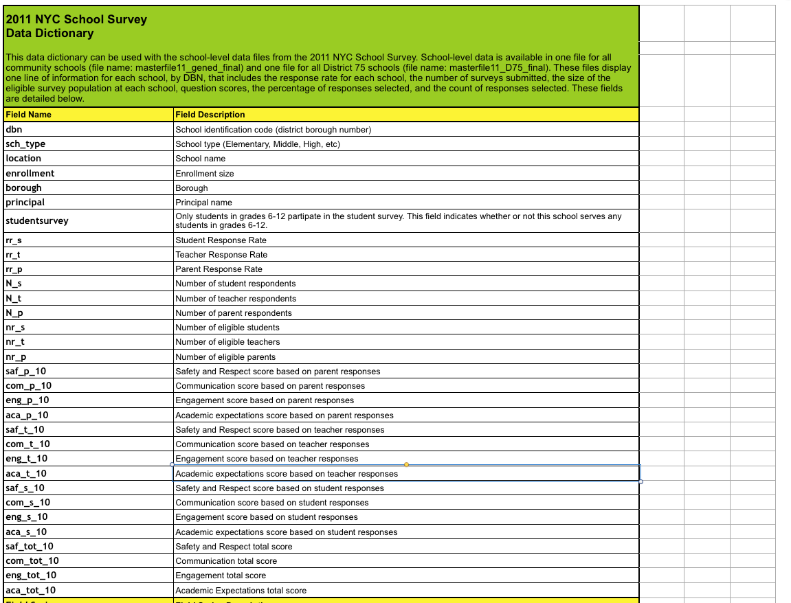
And then we remove all non-related columns in the survey:
In [17]: survey["DBN"] = survey["dbn"] survey_fields = ["DBN", "rr_s", "rr_t", "rr_p", "N_s", "N_t", "N_p", "saf_p_11", "com_p_11", "eng_p_11", "aca_p_11", "saf_t_11", "com_t_11", "eng_t_10", "aca_t_11", "saf_s_11", "com_s_11", "eng_s_11", "aca_s_11", "saf_tot_11", "com_tot_11", "eng_tot_11", "aca_tot_11",] survey = survey.loc[:,survey_fields] data["survey"] = survey survey.shape Out[17]: (1702, 23) Understanding exactly what each dataset contains and which columns from it are important can save a lot of time and effort later.
We condense datasets
If we take a look at some datasets, including class_size , we will immediately see the problem:
In [18]: data["class_size"].head() Out[18]: | CSD | BOROUGH | SCHOOL CODE | SCHOOL NAME | GRADE | PROGRAM TYPE | CORE SUBJECT (MS CORE and 9-12 ONLY) | / | |
|---|---|---|---|---|---|---|---|---|
| 0 | one | M | M015 | PS 015 Roberto Clemente | 0K | GEN ED | - | |
| one | one | M | M015 | PS 015 Roberto Clemente | 0K | CTT | - | |
| 2 | one | M | M015 | PS 015 Roberto Clemente | 01 | GEN ED | - | |
| 3 | one | M | M015 | PS 015 Roberto Clemente | 01 | CTT | - | |
| four | one | M | M015 | PS 015 Roberto Clemente | 02 | GEN ED | - |
| CORE COURSE (MS CORE and 9-12 ONLY) | SERVICE CATEGORY (K-9 * ONLY) | NUMBER OF STUDENTS / SEATS FILLED | NUMBER OF SECTIONS | AVERAGE CLASS SIZE | / | |
|---|---|---|---|---|---|---|
| 0 | - | - | 19.0 | 1.0 | 19.0 | |
| one | - | - | 21.0 | 1.0 | 21.0 | |
| 2 | - | - | 17.0 | 1.0 | 17.0 | |
| 3 | - | - | 17.0 | 1.0 | 17.0 | |
| four | - | - | 15.0 | 1.0 | 15.0 |
| SIZE OF SMALLEST CLASS | SIZE OF LARGEST CLASS | DATA SOURCE | SCHOOLWIDE PUPIL-TEACHER RATIO | DBN | |
|---|---|---|---|---|---|
| 0 | 19.0 | 19.0 | Ats | NaN | 01M015 |
| one | 21.0 | 21.0 | Ats | NaN | 01M015 |
| 2 | 17.0 | 17.0 | Ats | NaN | 01M015 |
| 3 | 17.0 | 17.0 | Ats | NaN | 01M015 |
| four | 15.0 | 15.0 | Ats | NaN | 01M015 |
There are several lines for each school (which can be understood by repeating DBN and SCHOOL NAME fields). Although, if we take a look at sat_results , there is only one line per school:
In [21]: data["sat_results"].head() Out[21]: | DBN | SCHOOL NAME | Num of SAT Test Takers | SAT Critical Reading Avg. Score | SAT Math Avg. Score | SAT Writing Avg. Score | |
|---|---|---|---|---|---|---|
| 0 | 01M292 | HENRY STREET SCHOOL FOR INTERNATIONAL STUDIES | 29 | 355 | 404 | 363 |
| one | 01M448 | UNIVERSITY NEIGHBORHOOD HIGH SCHOOL | 91 | 383 | 423 | 366 |
| 2 | 01M450 | EAST SIDE COMMUNITY SCHOOL | 70 | 377 | 402 | 370 |
| 3 | 01M458 | FORSYTH SATELLITE ACADEMY | 7 | 414 | 401 | 359 |
| four | 01M509 | MARTA VALLE HIGH SCHOOL | 44 | 390 | 433 | 384 |
To combine these datasets, we need a way to compact class_size datasets so that they have one line for each high school. If it does not work out, it will not work out and compare the EGE estimates with the size of the class. We can achieve this by better understanding the data, and then making some aggregations.
According to class_size , it seems that GRADE and PROGRAM TYPE contain different grades for each school. By limiting each field to a single value, we will be able to drop all duplicate lines. In the code below, we:
- Select only those values from class_size, where the GRADE field is 09-12.
- Select only those values from class_size, where the PROGRAM TYPE field is GEN ED.
- Group class_size by DBN, and take the average for each column. In essence, we will find an average class_size for each school.
- Drop the index so that the DBN is added again as a column.
In [68]: class_size = data["class_size"] class_size = class_size[class_size["GRADE "] == "09-12"] class_size = class_size[class_size["PROGRAM TYPE"] == "GEN ED"] class_size = class_size.groupby("DBN").agg(np.mean) class_size.reset_index(inplace=True) data["class_size"] = class_size We thicken the rest of the datasets
Next we need to shrink the demographics . Data collected over several years for the same schools. We will select only those lines where the schoolyear field is the freshest of all.
In [69]: demographics = data["demographics"] demographics = demographics[demographics["schoolyear"] == 20112012] data["demographics"] = demographics Now we need to compress math_test_results . It is divided by the Grade and Year values. We can choose a single class for a single year:
In [70]: data["math_test_results"] = data["math_test_results"][data["math_test_results"]["Year"] == 2011] data["math_test_results"] = data["math_test_results"][data["math_test_results"]["Grade"] == Finally, graduation also needs to be condensed:
In [71]: data["graduation"] = data["graduation"][data["graduation"]["Cohort"] == "2006"] data["graduation"] = data["graduation"][data["graduation"]["Demographic"] == "Total Cohort"] Cleaning and researching data is critical before working on the core of the project. Good, fit holistic dataset help make analysis faster.
Calculation of aggregated variables
The calculation of variables can speed up our analysis with the ability to make comparisons faster and, in principle, making it possible to do some comparisons that are impossible without them. The first thing we can do is calculate the total exam score from the individual columns of the SAT Math Avg. Score , SAT Critical Reading Avg. Score , and SAT Writing Avg. Score . In the code below, we:
- We transform each grade exam from line to number
- Add all the columns and get the sat_score column, the total score of the Unified State Exam.
In [72]: cols = ['SAT Math Avg. Score', 'SAT Critical Reading Avg. Score', 'SAT Writing Avg. Score'] for c in cols: data["sat_results"][c] = data["sat_results"][c].convert_objects(convert_numeric=True) data['sat_results']['sat_score'] = data['sat_results'][cols[0]] + data['sat_results'][cols[1]] Next we need to parse the coordinates of each school to make maps. They will allow us to mark the position of each school. In the code we:
- Break into latitude and longitude columns Location 1 column
- We convert lat and lon to numbers.
Let's output our datasets, see what happened:
In [74]: for k,v in data.items(): print(k) print(v.head()) math_test_results
| DBN | Grade | Year | Category | Number Tested | Mean Scale Score | \ | |
|---|---|---|---|---|---|---|---|
| 111 | 01M034 | eight | 2011 | All students | 48 | 646 | |
| 280 | 01M140 | eight | 2011 | All students | 61 | 665 | |
| 346 | 01M184 | eight | 2011 | All students | 49 | 727 | |
| 388 | 01M188 | eight | 2011 | All students | 49 | 658 | |
| 411 | 01M292 | eight | 2011 | All students | 49 | 650 |
| Level 1 # | Level 1% | Level 2 # | Level 2% | Level 3 # | Level 3% | Level 4 # | \ | |
|---|---|---|---|---|---|---|---|---|
| 111 | 15 | 31.3% | 22 | 45.8% | eleven | 22.9% | 0 | |
| 280 | one | 1.6% | 43 | 70.5% | 17 | 27.9% | 0 | |
| 346 | 0 | 0% | 0 | 0% | five | 10.2% | 44 | |
| 388 | ten | 20.4% | 26 | 53.1% | ten | 20.4% | 3 | |
| 411 | 15 | 30.6% | 25 | 51% | 7 | 14.3% | 2 |
| Level 4% | Level 3 + 4 # | Level 3 + 4% | |
|---|---|---|---|
| 111 | 0% | eleven | 22.9% |
| 280 | 0% | 17 | 27.9% |
| 346 | 89.8% | 49 | 100% |
| 388 | 6.1% | 13 | 26.5% |
| 411 | 4.1% | 9 | 18.4% |
survey
| DBN | rr_s | rr_t | rr_p | N_s | N_t | N_p | saf_p_11 | com_p_11 | eng_p_11 | \ | |
|---|---|---|---|---|---|---|---|---|---|---|---|
| 0 | 01M015 | NaN | 88 | 60 | NaN | 22.0 | 90.0 | 8.5 | 7.6 | 7.5 | |
| one | 01M019 | NaN | 100 | 60 | NaN | 34.0 | 161.0 | 8.4 | 7.6 | 7.6 | |
| 2 | 01M020 | NaN | 88 | 73 | NaN | 42.0 | 367.0 | 8.9 | 8.3 | 8.3 | |
| 3 | 01M034 | 89.0 | 73 | 50 | 145.0 | 29.0 | 151.0 | 8.8 | 8.2 | 8.0 | |
| four | 01M063 | NaN | 100 | 60 | NaN | 23.0 | 90.0 | 8.7 | 7.9 | 8.1 |
| ... | eng_t_10 | aca_t_11 | saf_s_11 | com_s_11 | eng_s_11 | aca_s_11 | \ | |
|---|---|---|---|---|---|---|---|---|
| 0 | ... | NaN | 7.9 | NaN | NaN | NaN | NaN | |
| one | ... | NaN | 9.1 | NaN | NaN | NaN | NaN | |
| 2 | ... | NaN | 7.5 | NaN | NaN | NaN | NaN | |
| 3 | ... | NaN | 7.8 | 6.2 | 5.9 | 6.5 | 7.4 | |
| four | ... | NaN | 8.1 | NaN | NaN | NaN | NaN |
| saf_tot_11 | com_tot_11 | eng_tot_11 | aca_tot_11 | |
|---|---|---|---|---|
| 0 | 8.0 | 7.7 | 7.5 | 7.9 |
| one | 8.5 | 8.1 | 8.2 | 8.4 |
| 2 | 8.2 | 7.3 | 7.5 | 8.0 |
| 3 | 7.3 | 6.7 | 7.1 | 7.9 |
| four | 8.5 | 7.6 | 7.9 | 8.0 |
ap_2010
| DBN | SchoolName | AP Test Takers | Total exams taken | Number of Exams with scores 3 4 or 5 | |
|---|---|---|---|---|---|
| 0 | 01M448 | UNIVERSITY NEIGHBORHOOD HS | 39 | 49 | ten |
| one | 01M450 | EAST SIDE COMMUNITY HS | nineteen | 21 | s |
| 2 | 01M515 | LOWER EASTSIDE PREP | 24 | 26 | 24 |
| 3 | 01M539 | NEW EXPLORATIONS SCI, TECH, MATH | 255 | 377 | 191 |
| four | 02M296 | High School of Hospitality Management | s | s | s |
sat_results
| DBN | SCHOOL NAME | Num of SAT Test Takers | SAT Critical Reading Avg. Score | \ | |
|---|---|---|---|---|---|
| 0 | 01M292 | HENRY STREET SCHOOL FOR INTERNATIONAL STUDIES | 29 | 355.0 | |
| one | 01M448 | UNIVERSITY NEIGHBORHOOD HIGH SCHOOL | 91 | 383.0 | |
| 2 | 01M450 | EAST SIDE COMMUNITY SCHOOL | 70 | 377.0 | |
| 3 | 01M458 | FORSYTH SATELLITE ACADEMY | 7 | 414.0 | |
| four | 01M509 | MARTA VALLE HIGH SCHOOL | 44 | 390.0 |
| SAT Math Avg. Score | SAT Writing Avg. Score | sat_score | |
|---|---|---|---|
| 0 | 404.0 | 363.0 | 1122.0 |
| one | 423.0 | 366.0 | 1172.0 |
| 2 | 402.0 | 370.0 | 1149.0 |
| 3 | 401.0 | 359.0 | 1174.0 |
| four | 433.0 | 384.0 | 1207.0 |
class_size
| DBN | CSD | NUMBER OF STUDENTS / SEATS FILLED | NUMBER OF SECTIONS | \ | |
|---|---|---|---|---|---|
| 0 | 01M292 | one | 88.0000 | 4.000000 | |
| one | 01M332 | one | 46.0000 | 2.000000 | |
| 2 | 01M378 | one | 33.0000 | 1.000000 | |
| 3 | 01M448 | one | 105.6875 | 4.750000 | |
| four | 01M450 | one | 57.6000 | 2.733333 |
| AVERAGE CLASS SIZE | SIZE OF SMALLEST CLASS | SIZE OF LARGEST CLASS | SCHOOLWIDE PUPIL-TEACHER RATIO | |
|---|---|---|---|---|
| 0 | 22.564286 | 18.50 | 26.571429 | NaN |
| one | 22.000000 | 21.00 | 23,500,000 | NaN |
| 2 | 33.000000 | 33.00 | 33.000000 | NaN |
| 3 | 22.231250 | 18.25 | 27.062500 | NaN |
| four | 21.200000 | 19.40 | 22.866667 | NaN |
demographics
| DBN | Name | schoolyear | \ | |
|---|---|---|---|---|
| 6 | 01M015 | PS 015 ROBERTO CLEMENTE | 20112012 | |
| 13 | 01M019 | PS 019 ASHER LEVY | 20112012 | |
| 20 | 01M020 | PS 020 ANNA SILVER | 20112012 | |
| 27 | 01M034 | PS 034 FRANKLIN D ROOSEVELT | 20112012 | |
| 35 | 01M063 | PS 063 WILLIAM MCKINLEY | 20112012 |
| fl_percent | frl_percent | total_enrollment | prek | k | grade1 | grade2 | \ | |
|---|---|---|---|---|---|---|---|---|
| 6 | NaN | 89.4 | 189 | 13 | 31 | 35 | 28 | |
| 13 | NaN | 61.5 | 328 | 32 | 46 | 52 | 54 | |
| 20 | NaN | 92.5 | 626 | 52 | 102 | 121 | 87 | |
| 27 | NaN | 99.7 | 401 | 14 | 34 | 38 | 36 | |
| 35 | NaN | 78.9 | 176 | 18 | 20 | thirty | 21 |
| ... | black_num | black_per | hispanic_num | hispanic_per | white_num | \ | |
|---|---|---|---|---|---|---|---|
| 6 | ... | 63 | 33.3 | 109 | 57.7 | four | |
| 13 | ... | 81 | 24.7 | 158 | 48.2 | 28 | |
| 20 | ... | 55 | 8.8 | 357 | 57.0 | sixteen | |
| 27 | ... | 90 | 22.4 | 275 | 68.6 | eight | |
| 35 | ... | 41 | 23.3 | 110 | 62.5 | 15 |
| white_per | male_num | male_per | female_num | female_per | |
|---|---|---|---|---|---|
| 6 | 2.1 | 97.0 | 51.3 | 92.0 | 48.7 |
| 13 | 8.5 | 147.0 | 44.8 | 181.0 | 55.2 |
| 20 | 2.6 | 330.0 | 52.7 | 296.0 | 47.3 |
| 27 | 2.0 | 204.0 | 50.9 | 197.0 | 49.1 |
| 35 | 8.5 | 97.0 | 55.1 | 79.0 | 44.9 |
graduation
| Demographic | DBN | School name | Cohort | \ | |
|---|---|---|---|---|---|
| 3 | Total cohort | 01M292 | HENRY STREET SCHOOL FOR INTERNATIONAL | 2006 | |
| ten | Total cohort | 01M448 | UNIVERSITY NEIGHBORHOOD HIGH SCHOOL | 2006 | |
| 17 | Total cohort | 01M450 | EAST SIDE COMMUNITY SCHOOL | 2006 | |
| 24 | Total cohort | 01M509 | MARTA VALLE HIGH SCHOOL | 2006 | |
| 31 | Total cohort | 01M515 | LOWER EAST SIDE PREPARATORY HIGH SCHO | 2006 |
| Total cohort | Total Grads - n | Total Grads -% of cohort | Total Regents - n | \ | |
|---|---|---|---|---|---|
| 3 | 78 | 43 | 55.1% | 36 | |
| ten | 124 | 53 | 42.7% | 42 | |
| 17 | 90 | 70 | 77.8% | 67 | |
| 24 | 84 | 47 | 56% | 40 | |
| 31 | 193 | 105 | 54.4% | 91 |
| Total Regents -% of cohort | Total Regents -% of grads | ... | Regents w / o Advanced - n | \ | |
|---|---|---|---|---|---|
| 3 | 46.2% | 83.7% | ... | 36 | |
| ten | 33.9% | 79.2% | ... | 34 | |
| 17 | 74.400000000000006% | 95.7% | ... | 67 | |
| 24 | 47.6% | 85.1% | ... | 23 | |
| 31 | 47.2% | 86.7% | ... | 22 |
| Regents w / o Advanced -% of cohort | Regents w / o Advanced -% of grads | \ | |
|---|---|---|---|
| 3 | 46.2% | 83.7% | |
| ten | 27.4% | 64.2% | |
| 17 | 74.400000000000006% | 95.7% | |
| 24 | 27.4% | 48.9% | |
| 31 | 11.4% | 21% |
| Local - n | Local -% of cohort | Local -% of grads | Still Enrolled - n | \ | |
|---|---|---|---|---|---|
| 3 | 7 | 9% | 16.3% | sixteen | |
| ten | eleven | 8.9% | 20.8% | 46 | |
| 17 | 3 | 3.3% | 4.3% | 15 | |
| 24 | 7 | 8.300000000000001% | 14.9% | 25 | |
| 31 | 14 | 7.3% | 13.3% | 53 |
| Still Enrolled -% of cohort | Dropped Out - n | Dropped Out -% of cohort | |
|---|---|---|---|
| 3 | 20.5% | eleven | 14.1% |
| ten | 37.1% | 20 | 16.100000000000001% |
| 17 | 16.7% | five | 5.6% |
| 24 | 29.8% | five | 6% |
| 31 | 27.5% | 35 | 18.100000000000001% |
hs_directory
| dbn | school_name | boro | \ | |
|---|---|---|---|---|
| 0 | 17K548 | Brooklyn School for Music & Theater | Brooklyn | |
| one | 09X543 | High School for Violin and Dance | Bronx | |
| 2 | 09X327 | Comprehensive Model School Project MS 327 | Bronx | |
| 3 | 02M280 | Manhattan Early College School for Advertising | Manhattan | |
| four | 28Q680 | Queens Gateway to Health Sciences Secondary Sc ... | Queens |
| building_code | phone_number | fax_number | grade_span_min | grade_span_max | \ | |
|---|---|---|---|---|---|---|
| 0 | K440 | 718-230-6250 | 718-230-6262 | 9 | 12 | |
| one | X400 | 718-842-0687 | 718-589-9849 | 9 | 12 | |
| 2 | X240 | 718-294-8111 | 718-294-8109 | 6 | 12 | |
| 3 | M520 | 718-935-3477 | NaN | 9 | ten | |
| four | Q695 | 718-969-3155 | 718-969-3552 | 6 | 12 |
| expgrade_span_min | expgrade_span_max | ... | priority05 | priority06 | priority07 | priority08 | \ | |
|---|---|---|---|---|---|---|---|---|
| 0 | NaN | NaN | ... | NaN | NaN | NaN | NaN | |
| one | NaN | NaN | ... | NaN | NaN | NaN | NaN | |
| 2 | NaN | NaN | ... | Then to New York City residents | NaN | NaN | NaN | |
| 3 | 9 | 14.0 | ... | NaN | NaN | NaN | NaN | |
| four | NaN | NaN | ... | NaN | NaN | NaN | NaN |
| priority09 | priority10 | Location 1 | \ | |
|---|---|---|---|---|
| 0 | NaN | NaN | 883 Classon Avenue \ nBrooklyn, NY 11225 \ n (40.67 ... | |
| one | NaN | NaN | 1110 Boston Road \ nBronx, NY 10456 \ n (40.8276026 ... | |
| 2 | NaN | NaN | 1501 Jerome Avenue \ nBronx, NY 10452 \ n (40.84241 ... | |
| 3 | NaN | NaN | 411 Pearl Street \ nNew York, NY 10038 \ n (40.7106 ... | |
| four | NaN | NaN | 160-20 Goethals Avenue \ nJamaica, NY 11432 (40 ... |
| DBN | lat | lon | |
|---|---|---|---|
| 0 | 17K548 | 40.670299 | -73.961648 |
| one | 09X543 | 40.827603 | -73.904475 |
| 2 | 09X327 | 40.842414 | -73.916162 |
| 3 | 02M280 | 40.710679 | -74.000807 |
| four | 28Q680 | 40.718810 | -73.806500 |
We combine datasets
After all the preparation, finally, we can merge all datasets on the DBN column. As a result, we get datasets with hundreds of columns, from all the original. When merging it is important to note that in some datasets there are no schools that are in sat_results dataset . To get around this, we need to merge datasets through the outer join, then we will not lose data. In the real analysis, the lack of data is common. Demonstrating the ability to explore and cope with such a lack is an important part of the portfolio.
You can read about different types of joins here .
In the code below, we:
- Let's go through all the elements of the data dictionary
- We derive the number of non-unique DBNs in each
- Decide how to join - internally or externally.
- Combine item with full dataframe through DBN column.
In [75]: flat_data_names = [k for k,v in data.items()] flat_data = [data[k] for k in flat_data_names] full = flat_data[0] for i, f in enumerate(flat_data[1:]): name = flat_data_names[i+1] print(name) print(len(f["DBN"]) - len(f["DBN"].unique())) join_type = "inner" if name in ["sat_results", "ap_2010", "graduation"]: join_type = "outer" if name not in ["math_test_results"]: full = full.merge(f, on="DBN", how=join_type) full.shape survey 0 ap_2010 1 sat_results 0 class_size 0 demographics 0 graduation 0 hs_directory 0 Out[75]: (374, 174) Add values
Now that we have our full full data frame, we have almost all the information for our analysis. Although there are still missing parts. We may want to correlate the test scores with the in-depth program with the USE estimates, but first we need to convert these columns to numbers, and then fill in all the missing values:
In [76]: cols = ['AP Test Takers ', 'Total Exams Taken', 'Number of Exams with scores 3 4 or 5'] for col in cols: full[col] = full[col].convert_objects(convert_numeric=True) full[cols] = full[cols].fillna(value=0) Next, you need to count the school_dist column, which indicates the school district. It will allow us to compare school districts and draw district statistics using the maps of the districts that we downloaded:
In [77]: full["school_dist"] = full["DBN"].apply(lambda x: x[:2]) Finally, we need to fill in all the missing values in full with the average value from the column in order to calculate the correlations
In [79]: full = full.fillna(full.mean()) We consider correlation
A good way to look at the datasets and see how the columns relate to what they need is to calculate the correlations. This will show which columns are associated with the column of interest. This can be done using the corr method in Pandas data frames. The closer the correlation is to 0, the weaker the connection. The closer to 1, the stronger the direct connection. The closer to -1, the stronger the feedback:
In [80]: full.corr()['sat_score'] Out[80]: Year NaN Number Tested 8.127817e-02 rr_s 8.484298e-02 rr_t -6.604290e-02 rr_p 3.432778e-02 N_s 1.399443e-01 N_t 9.654314e-03 N_p 1.397405e-01 saf_p_11 1.050653e-01 com_p_11 2.107343e-02 eng_p_11 5.094925e-02 aca_p_11 5.822715e-02 saf_t_11 1.206710e-01 com_t_11 3.875666e-02 eng_t_10 NaN aca_t_11 5.250357e-02 saf_s_11 1.054050e-01 com_s_11 4.576521e-02 eng_s_11 6.303699e-02 aca_s_11 8.015700e-02 saf_tot_11 1.266955e-01 com_tot_11 4.340710e-02 eng_tot_11 5.028588e-02 aca_tot_11 7.229584e-02 AP Test Takers 5.687940e-01 Total Exams Taken 5.585421e-01 Number of Exams with scores 3 4 or 5 5.619043e-01 SAT Critical Reading Avg. Score 9.868201e-01 SAT Math Avg. Score 9.726430e-01 SAT Writing Avg. Score 9.877708e-01 ... SIZE OF SMALLEST CLASS 2.440690e-01 SIZE OF LARGEST CLASS 3.052551e-01 SCHOOLWIDE PUPIL-TEACHER RATIO NaN schoolyear NaN frl_percent -7.018217e-01 total_enrollment 3.668201e-01 ell_num -1.535745e-01 ell_percent -3.981643e-01 sped_num 3.486852e-02 sped_percent -4.413665e-01 asian_num 4.748801e-01 asian_per 5.686267e-01 black_num 2.788331e-02 black_per -2.827907e-01 hispanic_num 2.568811e-02 hispanic_per -3.926373e-01 white_num 4.490835e-01 white_per 6.100860e-01 male_num 3.245320e-01 male_per -1.101484e-01 female_num 3.876979e-01 female_per 1.101928e-01 Total Cohort 3.244785e-01 grade_span_max -2.495359e-17 expgrade_span_max NaN zip -6.312962e-02 total_students 4.066081e-01 number_programs 1.166234e-01 lat -1.198662e-01 lon -1.315241e-01 Name: sat_score, dtype: float64 This data gives us a number of hints that need to be worked out:
- The total number of classes ( total_enrollment ) strongly correlates with the USE grades ( sat_score ), which is surprising because, at first glance, small schools that work better with individual students should have higher marks.
- The percentage of women in school ( female_per ) is positively correlated with the exam scores, while the percentage of men ( male_per ) is negative.
- None of the survey results correlate strongly with the USE estimates.
- There is a significant racial inequality in the USE estimates ( white_per , asian_per , black_per , hispanic_per ).
- ell_percent strongly correlates in the opposite direction with EGE estimates.
Each item is a potential place for research and history based on data.
Just in case, let me remind you that the correlation (and covariance) show only a measure of linear dependence. If there is a connection, but not a linear one, say, a quadratic one - the correlation will not show anything sensible.
And, of course, the correlation in no way indicates a cause and effect. It is simply that the two quantities tend to change in proportion. Below is just an example of the search for a valid pattern and analyzed.
We define the context
Before diving into the study of data, it would be necessary to define the context, both for ourselves and for those who will read our analysis later. A good way - research charts or maps. In our case, we will draw on the map the location of our schools, which will help readers to understand the problem we are studying.
In the code below, we:
- Prepare a map of New York
- Add a marker to the map for each school in the city.
- Draw a map
In [82]: import folium from folium import plugins schools_map = folium.Map(location=[full['lat'].mean(), full['lon'].mean()], zoom_start=10) marker_cluster = folium.MarkerCluster().add_to(schools_map) for name, row in full.iterrows(): folium.Marker([row["lat"], row["lon"]], popup="{0}: {1}".format(row["DBN"], row["school_name"])).add_to(marker_cluster) schools_map.create_map('schools.html') schools_map Out[82]: 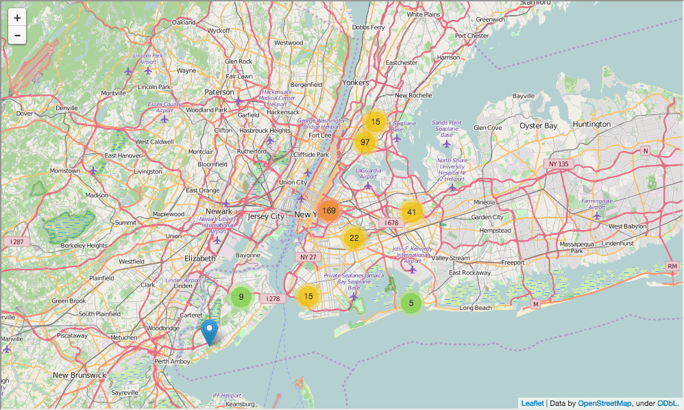
, , - . :
In [84]: schools_heatmap = folium.Map(location=[full['lat'].mean(), full['lon'].mean()], zoom_start=10) schools_heatmap.add_children(plugins.HeatMap([[row["lat"], row["lon"]] for name, row in full.iterrows()])) schools_heatmap.save("heatmap.html") schools_heatmap Out[84]: 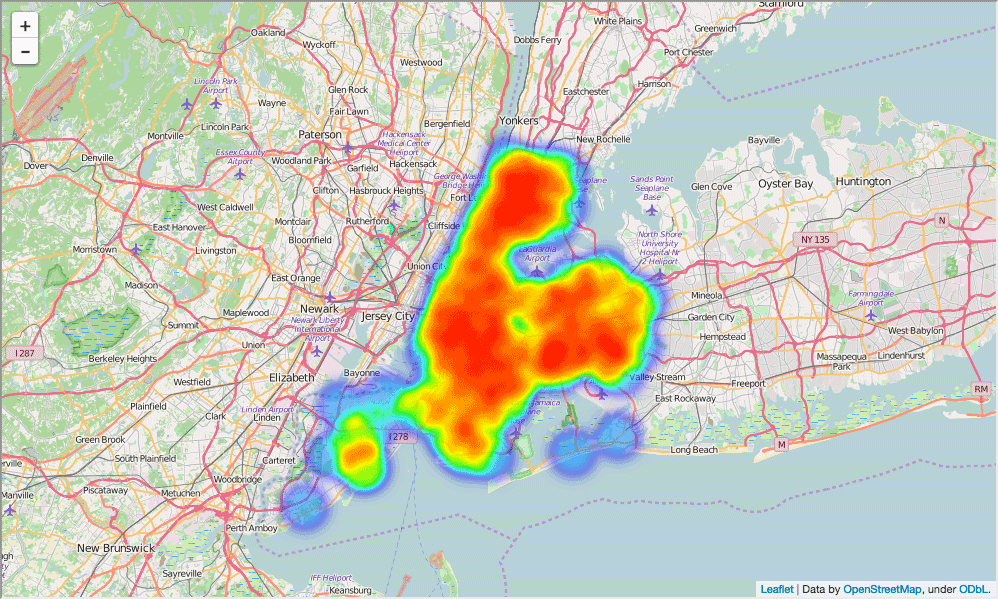
, - , . , .. . - , .
. :
- full
- school_dist , ,
In [ ]: district_data = full.groupby("school_dist").agg(np.mean) district_data.reset_index(inplace=True) district_data["school_dist"] = district_data["school_dist"].apply(lambda x: str(int(x)) . GeoJSON , , school_dist , , , .
In [85]: def show_district_map(col): geo_path = 'schools/districts.geojson' districts = folium.Map(location=[full['lat'].mean(), full['lon'].mean()], zoom_start=10) districts.geo_json( geo_path=geo_path, data=district_data, columns=['school_dist', col], key_on='feature.properties.school_dist', fill_color='YlGn', fill_opacity=0.7, line_opacity=0.2, ) districts.save("districts.html") return districts show_district_map("sat_score") Out[85]: 
, ; , . , , . — , , .
, :
In [87]: %matplotlib inline full.plot.scatter(x='total_enrollment', y='sat_score') Out[87]: <matplotlib.axes._subplots.AxesSubplot at 0x10fe79978> 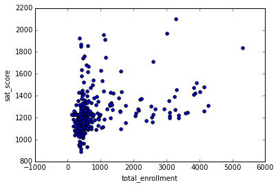
, . , . .
, :
In [88]: full[(full["total_enrollment"] < 1000) & (full["sat_score"] < 1000)]["School Name"] Out[88]: 34 INTERNATIONAL SCHOOL FOR LIBERAL ARTS 143 NaN 148 KINGSBRIDGE INTERNATIONAL HIGH SCHOOL 203 MULTICULTURAL HIGH SCHOOL 294 INTERNATIONAL COMMUNITY HIGH SCHOOL 304 BRONX INTERNATIONAL HIGH SCHOOL 314 NaN 317 HIGH SCHOOL OF WORLD CULTURES 320 BROOKLYN INTERNATIONAL HIGH SCHOOL 329 INTERNATIONAL HIGH SCHOOL AT PROSPECT 331 IT TAKES A VILLAGE ACADEMY 351 PAN AMERICAN INTERNATIONAL HIGH SCHOO Name: School Name, dtype: object , , , , , . , — , , .
, , . ell_percent - . :
In [89]: full.plot.scatter(x='ell_percent', y='sat_score') Out[89]: <matplotlib.axes._subplots.AxesSubplot at 0x10fe824e0> 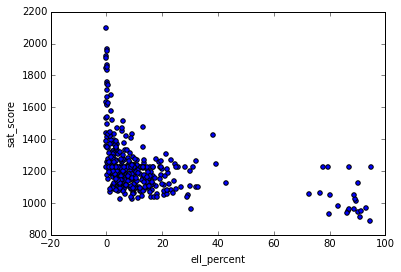
, ell_percentage . , , :
In [90]: show_district_map("ell_percent") Out[90]: 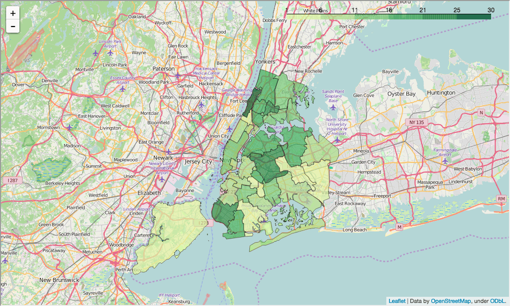
, , .
, , . , . :
In [91]: full.corr()["sat_score"][["rr_s", "rr_t", "rr_p", "N_s", "N_t", "N_p", "saf_tot_11", "com_tot_11", "aca_tot_11", "eng_tot_11"]].plot.bar() Out[91]: <matplotlib.axes._subplots.AxesSubplot at 0x114652400> 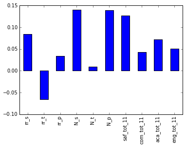
, N_p N_s , . , ell_learners . — saf_t_11 . , , . , , — . , , , , . , - , ( — , ).
. , , :
In [92]: full.corr()["sat_score"][["white_per", "asian_per", "black_per", "hispanic_per"]].plot.bar() Out[92]: <matplotlib.axes._subplots.AxesSubplot at 0x108166ba8> 
, , . , , . , :
In [93]: show_district_map("hispanic_per") Out[93]: 
, - , .
— . , . :
In [94]: full.corr()["sat_score"][["male_per", "female_per"]].plot.bar() Out[94]: <matplotlib.axes._subplots.AxesSubplot at 0x10774d0f0> 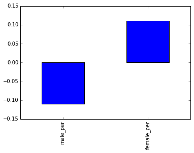
, female_per sat_score :
In [95]: full.plot.scatter(x='female_per', y='sat_score') Out[95]: <matplotlib.axes._subplots.AxesSubplot at 0x104715160> 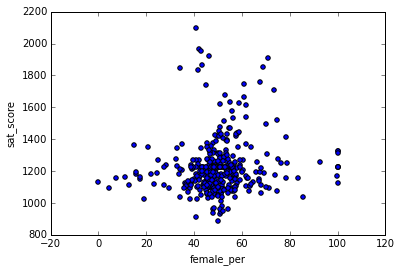
, ( ). :
In [96]: full[(full["female_per"] > 65) & (full["sat_score"] > 1400)]["School Name"] Out[96]: 3 PROFESSIONAL PERFORMING ARTS HIGH SCH 92 ELEANOR ROOSEVELT HIGH SCHOOL 100 TALENT UNLIMITED HIGH SCHOOL 111 FIORELLO H. LAGUARDIA HIGH SCHOOL OF 229 TOWNSEND HARRIS HIGH SCHOOL 250 FRANK SINATRA SCHOOL OF THE ARTS HIGH SCHOOL 265 BARD HIGH SCHOOL EARLY COLLEGE Name: School Name, dtype: object , , . . , , , , , .
, 100 ( ).
. , — , , . , , .
In [98]: full["ap_avg"] = full["AP Test Takers "] / full["total_enrollment"] full.plot.scatter(x='ap_avg', y='sat_score') Out[98]: <matplotlib.axes._subplots.AxesSubplot at 0x11463a908> 
, . , :
In [99]: full[(full["ap_avg"] > .3) & (full["sat_score"] > 1700)]["School Name"] Out[99]: 92 ELEANOR ROOSEVELT HIGH SCHOOL 98 STUYVESANT HIGH SCHOOL 157 BRONX HIGH SCHOOL OF SCIENCE 161 HIGH SCHOOL OF AMERICAN STUDIES AT LE 176 BROOKLYN TECHNICAL HIGH SCHOOL 229 TOWNSEND HARRIS HIGH SCHOOL 243 QUEENS HIGH SCHOOL FOR THE SCIENCES A 260 STATEN ISLAND TECHNICAL HIGH SCHOOL Name: School Name, dtype: object , , , . , .
data science - . , . , , , .
— . — - . — , .
, , . :)
What's next
— , .
Dataquest , , . — .
')
Source: https://habr.com/ru/post/331528/
All Articles