Autoencoders in Keras, Part 2: Manifold learning and latent variables
Content
- Part 1: Introduction
- Part 2: Manifold learning and latent variables
- Part 3: Variational autoencoders ( VAE )
- Part 4: Conditional VAE
- Part 5: GAN (Generative Adversarial Networks) and tensorflow
- Part 6: VAE + GAN
In order to better understand how autoencoders work, and also to subsequently generate something new from codes, it is worth understanding what codes are and how they can be interpreted.
Manifold learning
Images of numbers mnist (in which examples in the last part) are elements
 -dimensional space, as in general, any monochrome image 28 to 28.
')
However, among all images, images of numbers occupy only a tiny part, the absolute majority of images are just noise.
On the other hand, if you take an arbitrary image of a digit, then all the images from a certain neighborhood can also be considered a digit.
And if you take two arbitrary images of a digit, then in the original 784-dimensional space you can most likely find a continuous curve, all points along which you can also be considered as numbers (at least for images of numbers of one label), and along with the previous remark, all points of some area along this curve.
Thus, in the space of all images there is a certain subspace of smaller dimension in the area around which the images of numbers are concentrated. That is, if our population is all images of numbers that can be drawn in principle, then the density of probability to meet such a figure within the region is much higher than outside.
Autoencoders with the dimension of code k are looking for a k-dimensional manifold in the space of objects, which most fully conveys all variations in the sample. And the code itself sets the parameterization of this manifold. In this case, the encoder associates an object with its parameter on a manifold, and the decoder associates a point in the object space with a parameter.
The larger the dimension of the codes, the more variations in the data the autoencoder can transmit. If the dimension of the codes is too small, the autoencoder will memorize something in between the missing variations in the given metric (this is one of the reasons why mnist numbers become more blurred as the code dimension decreases in the autoencoders).
In order to better understand what is manifold learning , we will create a simple two-dimensional dataset in the form of a curve plus noise and we will train an autoencoder on it.
Code and visualization
# import numpy as np import matplotlib.pyplot as plt %matplotlib inline import seaborn as sns # x1 = np.linspace(-2.2, 2.2, 1000) fx = np.sin(x1) dots = np.vstack([x1, fx]).T noise = 0.06 * np.random.randn(*dots.shape) dots += noise # from itertools import cycle size = 25 colors = ["r", "g", "c", "y", "m"] idxs = range(0, x1.shape[0], x1.shape[0]//size) vx1 = x1[idxs] vdots = dots[idxs] # plt.figure(figsize=(12, 10)) plt.xlim([-2.5, 2.5]) plt.scatter(dots[:, 0], dots[:, 1]) plt.plot(x1, fx, color="red", linewidth=4) plt.grid(False) 
In the picture above: the blue dots are the data, and the red curve is the variety that defines our data.
Linear compression autoencoder
The simplest autoencoder is a two-layer compression autoencoder with linear activation functions (more layers do not make sense with linear activation).
Such an autoencoder is looking for an affine (linear with a shift) subspace in the object space that describes the greatest variation in objects, the PCA (principal component method) does the same thing, and both of them find the same subspace
from keras.layers import Input, Dense from keras.models import Model from keras.optimizers import Adam def linear_ae(): input_dots = Input((2,)) code = Dense(1, activation='linear')(input_dots) out = Dense(2, activation='linear')(code) ae = Model(input_dots, out) return ae ae = linear_ae() ae.compile(Adam(0.01), 'mse') ae.fit(dots, dots, epochs=15, batch_size=30, verbose=0) # pdots = ae.predict(dots, batch_size=30) vpdots = pdots[idxs] # PCA from sklearn.decomposition import PCA pca = PCA(1) pdots_pca = pca.inverse_transform(pca.fit_transform(dots)) Visualization
# plt.figure(figsize=(12, 10)) plt.xlim([-2.5, 2.5]) plt.scatter(dots[:, 0], dots[:, 1], zorder=1) plt.plot(x1, fx, color="red", linewidth=4, zorder=10) plt.plot(pdots[:,0], pdots[:,1], color='white', linewidth=12, zorder=3) plt.plot(pdots_pca[:,0], pdots_pca[:,1], color='orange', linewidth=4, zorder=4) plt.scatter(vpdots[:,0], vpdots[:,1], color=colors*5, marker='*', s=150, zorder=5) plt.scatter(vdots[:,0], vdots[:,1], color=colors*5, s=150, zorder=6) plt.grid(False) 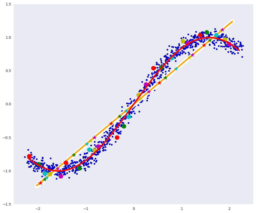
In the picture above:
- the white line is the manifold to which the blue data points after the autoencoder go, that is, the autoencoder's attempt to construct the manifold that determines the most variations in the data,
- the orange line is the manifold to which the blue data points go after the PCA,
- colored circles are points that turn into asterisks of the corresponding color after the autoencoder,
- multi-colored asterisks - respectively, the images of circles after the auto-encoder.
An autoencoder looking for linear dependencies may not be as useful as an autoencoder, which can find arbitrary dependencies in data. It would be useful if both the encoder and the decoder could approximate arbitrary functions. If both the encoder and the decoder are added at least one layer of sufficient size and a non-linear activation function between them, they can find arbitrary dependencies.
Deep autoencoder
A deep autoencoder has more layers and the most important is a non-linear activation function between them (in our case, ELU is the Exponential Linear Unit).
def deep_ae(): input_dots = Input((2,)) x = Dense(64, activation='elu')(input_dots) x = Dense(64, activation='elu')(x) code = Dense(1, activation='linear')(x) x = Dense(64, activation='elu')(code) x = Dense(64, activation='elu')(x) out = Dense(2, activation='linear')(x) ae = Model(input_dots, out) return ae dae = deep_ae() dae.compile(Adam(0.003), 'mse') dae.fit(dots, dots, epochs=200, batch_size=30, verbose=0) pdots_d = dae.predict(dots, batch_size=30) vpdots_d = pdots_d[idxs] Visualization
# plt.figure(figsize=(12, 10)) plt.xlim([-2.5, 2.5]) plt.scatter(dots[:, 0], dots[:, 1], zorder=1) plt.plot(x1, fx, color="red", linewidth=4, zorder=10) plt.plot(pdots_d[:,0], pdots_d[:,1], color='white', linewidth=12, zorder=3) plt.plot(pdots_pca[:,0], pdots_pca[:,1], color='orange', linewidth=4, zorder=4) plt.scatter(vpdots_d[:,0], vpdots_d[:,1], color=colors*5, marker='*', s=150, zorder=5) plt.scatter(vdots[:,0], vdots[:,1], color=colors*5, s=150, zorder=6) plt.grid(False) 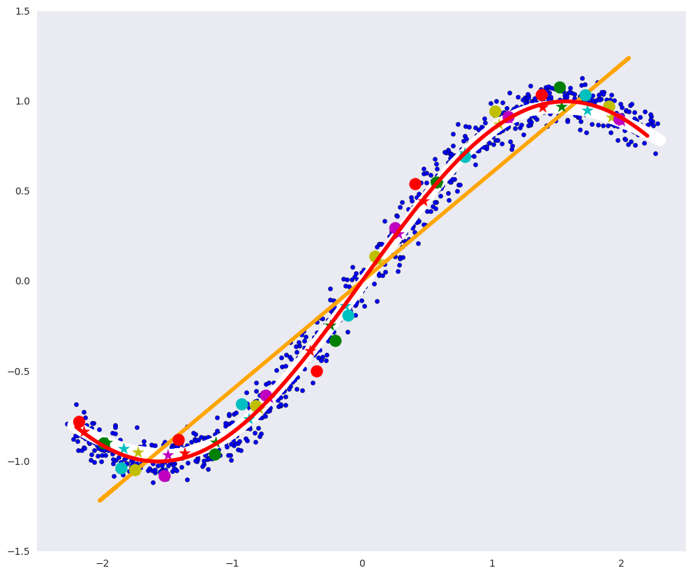
Such an autoencoder made it almost perfectly possible to build a defining manifold: the white curve almost coincides with the red one.
A deep autoencoder can theoretically find a variety of arbitrary complexity, for example, one about which numbers lie in a 784-dimensional space.
If we take two objects and look at objects lying on an arbitrary curve between them, then most likely intermediate objects will not belong to the general population, since the variety on which the general population lies may be highly curved and small.
Let's return to the handwritten numbers from the previous part.
First, we move in a straight line in the space of numbers from one bit to another:
Code
from keras.layers import Conv2D, MaxPooling2D, UpSampling2D from keras.datasets import mnist (x_train, y_train), (x_test, y_test) = mnist.load_data() x_train = x_train.astype('float32') / 255. x_test = x_test .astype('float32') / 255. x_train = np.reshape(x_train, (len(x_train), 28, 28, 1)) x_test = np.reshape(x_test, (len(x_test), 28, 28, 1)) # def create_deep_conv_ae(): input_img = Input(shape=(28, 28, 1)) x = Conv2D(128, (7, 7), activation='relu', padding='same')(input_img) x = MaxPooling2D((2, 2), padding='same')(x) x = Conv2D(32, (2, 2), activation='relu', padding='same')(x) x = MaxPooling2D((2, 2), padding='same')(x) encoded = Conv2D(1, (7, 7), activation='relu', padding='same')(x) # (7, 7, 1) .. 49- input_encoded = Input(shape=(7, 7, 1)) x = Conv2D(32, (7, 7), activation='relu', padding='same')(input_encoded) x = UpSampling2D((2, 2))(x) x = Conv2D(128, (2, 2), activation='relu', padding='same')(x) x = UpSampling2D((2, 2))(x) decoded = Conv2D(1, (7, 7), activation='sigmoid', padding='same')(x) # encoder = Model(input_img, encoded, name="encoder") decoder = Model(input_encoded, decoded, name="decoder") autoencoder = Model(input_img, decoder(encoder(input_img)), name="autoencoder") return encoder, decoder, autoencoder c_encoder, c_decoder, c_autoencoder = create_deep_conv_ae() c_autoencoder.compile(optimizer='adam', loss='binary_crossentropy') c_autoencoder.fit(x_train, x_train, epochs=50, batch_size=256, shuffle=True, validation_data=(x_test, x_test)) def plot_digits(*args): args = [x.squeeze() for x in args] n = min([x.shape[0] for x in args]) plt.figure(figsize=(2*n, 2*len(args))) for j in range(n): for i in range(len(args)): ax = plt.subplot(len(args), n, i*n + j + 1) plt.imshow(args[i][j]) plt.gray() ax.get_xaxis().set_visible(False) ax.get_yaxis().set_visible(False) plt.show() # def plot_homotopy(frm, to, n=10, decoder=None): z = np.zeros(([n] + list(frm.shape))) for i, t in enumerate(np.linspace(0., 1., n)): z[i] = frm * (1-t) + to * t if decoder: plot_digits(decoder.predict(z, batch_size=n)) else: plot_digits(z) # frm, to = x_test[y_test == 8][1:3] plot_homotopy(frm, to) 
If we move along a curve between the codes (and if the variety of codes is well parametrized), then the decoder will translate this curve from the code space to a curve that does not leave the defining manifold in the space of objects. That is, intermediate objects on the curve will belong to the entire population.
codes = c_encoder.predict(x_test[y_test == 8][1:3]) plot_homotopy(codes[0], codes[1], n=10, decoder=c_decoder) 
Intermediate figures - quite a good eight.
Thus, it can be said that the autoencoder, at least locally, learned the form of the defining manifold.
Reengineering autoencoder
In order for the autoencoder to learn how to isolate any complex patterns, the generalizing abilities of the encoder and decoder must be limited, otherwise even an autoencoder with a one-dimensional code can simply draw a one-dimensional curve through each point in the training set, i.e. just remember each object. But this complex manifold, which the autoencoder will build, will not have much in common with the manifold defining population.
Let's take the same problem with artificial data, train the same deep autoencoder on a very small subset of points and look at the resulting variety:
Code
dae = deep_ae() dae.compile(Adam(0.0003), 'mse') x_train_oft = np.vstack([dots[idxs]]*4000) dae.fit(x_train_oft, x_train_oft, epochs=200, batch_size=15, verbose=1) pdots_d = dae.predict(dots, batch_size=30) vpdots_d = pdots_d[idxs] plt.figure(figsize=(12, 10)) plt.xlim([-2.5, 2.5]) plt.scatter(dots[:, 0], dots[:, 1], zorder=1) plt.plot(x1, fx, color="red", linewidth=4, zorder=10) plt.plot(pdots_d[:,0], pdots_d[:,1], color='white', linewidth=6, zorder=3) plt.plot(pdots_pca[:,0], pdots_pca[:,1], color='orange', linewidth=4, zorder=4) plt.scatter(vpdots_d[:,0], vpdots_d[:,1], color=colors*5, marker='*', s=150, zorder=5) plt.scatter(vdots[:,0], vdots[:,1], color=colors*5, s=150, zorder=6) plt.grid(False) 
It can be seen that the white curve has passed through each data point and is slightly similar to the red curve defining the data: the face has a typical re-training.
Hidden variables
You can consider the population as some data generation process.
 which depends on a number of hidden variables.
  (random variables). Data dimension may be much higher than the dimension of hidden random variables which this data defines. Consider the process of generating regular numbers: how the figure will look can depend on many factors:
- desired digits
- stroke thickness
- tilt digits
- neatness
- etc.
Each of these factors has its own prior distribution, for example, the probability that a figure of eight will be drawn is the Bernoulli distribution with a probability of 1/10, the thickness of the stroke also has some distribution and may depend on both accuracy and its hidden variables, such as the thickness of the handle or the temperament of a person (again with their own distributions).
Autoencoder itself in the process of learning must come to hidden factors, for example, such as those listed above, some of their complex combinations, or in general to completely different ones. However, the joint distribution that he learns does not have to be simple, it can be some kind of complex curved area. (The decoder can also transfer values from outside this area, only the results will no longer be from the defining manifold, but from its random continuous continuation).
That's why we can't just generate new ones.
from the distribution of these hidden variables. It is difficult to remain within the region, and even harder to somehow interpret the values of the hidden variables in this curve region.For definiteness, we introduce some notation on the example of numbers:
- - random size of the picture 2828,
- - random value of hidden factors that determine the number in the picture,
 - the probability distribution of images of figures in pictures, i.e. the probability of a particular image of a digit is in principle to be drawn (if the picture is not like a digit, then this probability is extremely small),
 - the probability distribution of hidden factors, for example, the distribution of the thickness of the stroke,
 - probability distribution of hidden factors for a given picture (a different combination of hidden variables and noise can lead to the same picture),
 - the probability distribution of pictures for given hidden factors, the same factors can lead to different pictures (the same person in the same conditions does not draw absolutely identical numbers),
 - joint distribution and , the most complete understanding of the data needed to generate new objects.
 the decoder brings us closer but at the moment we still do not understand.
Let's see how the hidden variables are distributed in the usual autoencoder:
Code
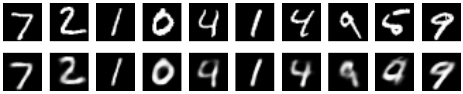
from keras.layers import Flatten, Reshape from keras.regularizers import L1L2 def create_deep_sparse_ae(lambda_l1): # encoding_dim = 16 # input_img = Input(shape=(28, 28, 1)) flat_img = Flatten()(input_img) x = Dense(encoding_dim*4, activation='relu')(flat_img) x = Dense(encoding_dim*3, activation='relu')(x) x = Dense(encoding_dim*2, activation='relu')(x) encoded = Dense(encoding_dim, activation='linear', activity_regularizer=L1L2(lambda_l1, 0))(x) # input_encoded = Input(shape=(encoding_dim,)) x = Dense(encoding_dim*2, activation='relu')(input_encoded) x = Dense(encoding_dim*3, activation='relu')(x) x = Dense(encoding_dim*4, activation='relu')(x) flat_decoded = Dense(28*28, activation='sigmoid')(x) decoded = Reshape((28, 28, 1))(flat_decoded) # encoder = Model(input_img, encoded, name="encoder") decoder = Model(input_encoded, decoded, name="decoder") autoencoder = Model(input_img, decoder(encoder(input_img)), name="autoencoder") return encoder, decoder, autoencoder encoder, decoder, autoencoder = create_deep_sparse_ae(0.) autoencoder.compile(optimizer=Adam(0.0003), loss='binary_crossentropy') autoencoder.fit(x_train, x_train, epochs=100, batch_size=64, shuffle=True, validation_data=(x_test, x_test)) n = 10 imgs = x_test[:n] decoded_imgs = autoencoder.predict(imgs, batch_size=n) plot_digits(imgs, decoded_imgs) Here are the images recovered by this encoder:
Images
Joint allocation of hidden variables

codes = encoder.predict(x_test) sns.jointplot(codes[:,1], codes[:,3]) 
It is seen that the joint distribution
has a complex shape;  and
and  addicted to each other.
Is there some way to control the distribution of hidden variables
 ?
?The easiest way is to add a regularizer
 or
or  on values , this will add a priori assumptions on the distribution of hidden variables, respectively, the laplass or normal (similar to the a priori distribution added to the values of the weights during regularization).
The regularizer forces the autoencoder to look for hidden variables that are distributed according to the necessary laws, whether it will work out is another question. However, this does not make them independent, i.e.
 .
.Let's look at the joint distribution of hidden parameters in a sparse autoencoder.
Code and visualization
s_encoder, s_decoder, s_autoencoder = create_deep_sparse_ae(0.00001) s_autoencoder.compile(optimizer=Adam(0.0003), loss='binary_crossentropy') s_autoencoder.fit(x_train, x_train, epochs=200, batch_size=256, shuffle=True, validation_data=(x_test, x_test)) imgs = x_test[:n] decoded_imgs = s_autoencoder.predict(imgs, batch_size=n) plot_digits(imgs, decoded_imgs) codes = s_encoder.predict(x_test) snt.jointplot(codes[:,1], codes[:,3])  and still dependent on each other, but now at least distributed around 0, and even more or less normal.
How to control the hidden space, so that you can intelligently generate images from it - in the next part about variational autoencoders (VAE).
Useful links and literature
This post is based on the chapter on autoencoders (in particular the subchapters of the Learning Maifolds with autoencoders ) in the Deep Learning Book .
Source: https://habr.com/ru/post/331500/
All Articles