Machine Learning for an Insurance Company: Exploring Algorithms
I propose to continue the good tradition that began on Friday just over a month ago. Then I shared with you an introductory article about why machine learning in an insurance company is needed and how the realism of the idea itself was tested. Today will be its continuation, in which the most interesting begins - the testing of algorithms.

1. Realistic ideas .
2. We investigate the algorithms .
3. Improving the model through algorithm optimization .
In the first article, we talked about the fact that Azure supports the use of Python scripts. The module required for this can receive as input two data arrays and a zip-archive with additional materials (for example, other scripts, libraries, etc.).
')
A simple example: in the first article in the final assessment, there was a remark about an unbalanced test sample in classes. You can correct the situation by entering into the scheme a simple script that will filter out extra lines in the entire sample. As a demonstration, we will do it in the following way (others are possible).

The module returns a modified data array, which (as will be seen later) contains an equal number of records for both classes.
In almost any machine learning task, the raw data does not provide a satisfactory result. To select the most informative features for the model, data mining is required.
In the prototype, which was discussed in the previous article, two types of data were used: the number of visits by the patient to the doctor in the last three months and the last amount spent on this visit. To begin, add:
However, in this way we will only increase the number of signs without having processed them in any way. To do this, we use MS Analysis Services, which uses machine learning to extract features, in particular, a simplified Bayesian algorithm.

Based on the results, you can select boundaries for the binary representation of the input data. For example, “age less than 19” and “number of visits to a doctor is less than 5” indicate a greater likelihood of no peak. While the “age is older than 64” and “the number of requests is more than 14” is fraught with expenses next month.
You can get a list of diagnoses, which most often precede large spending.
This is only part of the selected diagnoses. In each of the diagnoses, with a probability of from 85% to 100%, there will be a peak in costs. Their presence is worth making a separate sign. Do not miss the presence of conventional diagnoses, which will not cost the company expensive. Therefore, we should normalize the probabilities found and introduce a new sign, which will be a weighted sum of the number of diagnoses over the past 90 days.
As a result, seven parameters were obtained in the input feature vector. Compare them with what was obtained last time using different algorithms.
We will determine the parameters that will be used for training. Consider several different classification algorithms: logistic regression, support vector machine, decision jungle / random forest, Bayesian network. Neural networks are also an obvious option, but this is a separate complex topic and in this case this algorithm will be redundant.
Since the data was filtered to obtain a balanced sample, we will not change the boundary value for the assignment of classes. We will return to this question in the next article.
This is a special case of a linear regressor adapted to the tasks of classification. The algorithm was already mentioned in the first article, where it was used to build the simplest model as a prototype.
At the initial stage, it allows you to get the initial value in the range from minus to plus infinity. Next, we perform the transformation using a sigmoid function of the form 1 / (1 + e ^ (- score)), where score is the value obtained earlier, we perform the conversion. The result will be a number ranging from -1 to +1. The decision to belong to the class is made on the basis of the selected threshold value.
Options:

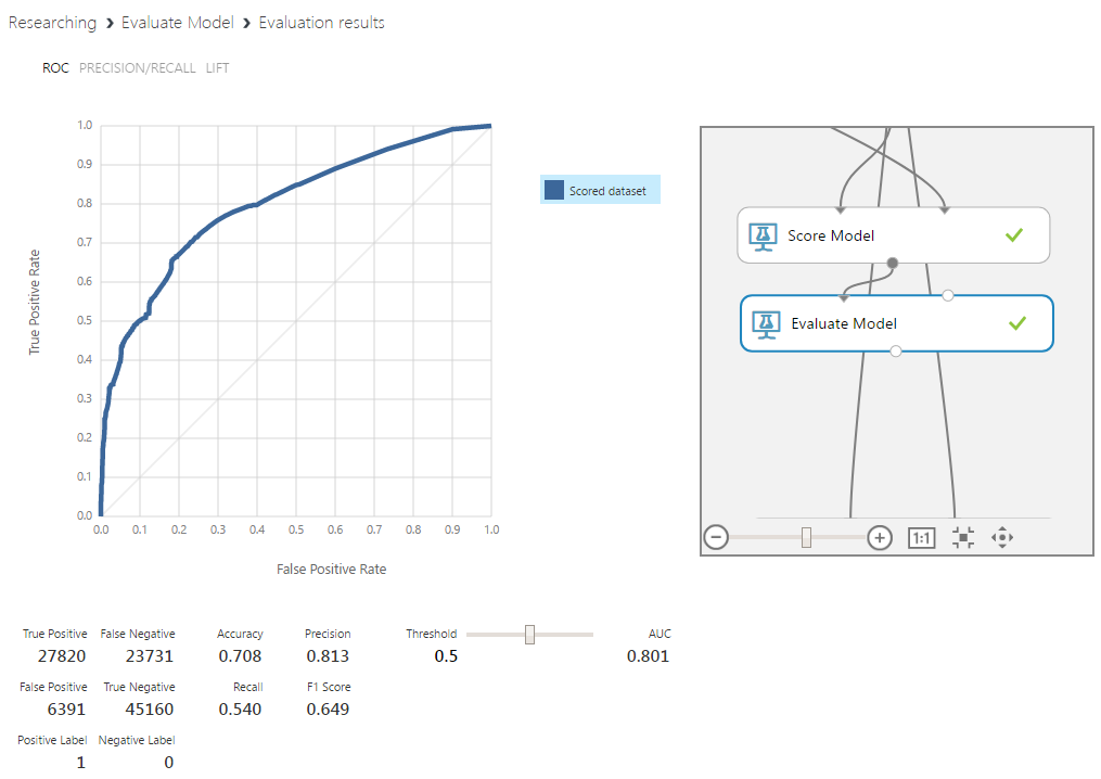
This algorithm was used in the prototype model, so the comparison will be most revealing. Even without adjusting the boundaries of the definition of classes and with small additions to the vector of input features, the percentage of correctly predicted peaks increased by 5%, and their absence increased by 15%. Such an important indicator, as the area under the curve of this graph, also increased significantly. This parameter reflects how well the values of classes relate to each other for different boundary values. The further the curve is from the diagonal, the better.
The support vector method is included in the group of linear classifiers, although some modifications to the main part of the algorithm allow the construction of non-linear classifiers. The bottom line is to translate the source data into a higher dimension and build a separating hyperplane. Increasing the dimensionality is necessary, since the source vectors are often linearly inseparable. After translation, the hyperplane is searched for with the condition of maximum clearance to hyperplanes, denoting the boundary of classes.

Options:

The graph shows that this is not the most successful algorithm for this task. Accuracy and area under the curve are low. In addition, the curve itself is unstable in nature, which might be acceptable for the prototype, but not for the model with the processed data.
Bayesian networks are a probabilistic data model, represented as an acyclic directed graph. The vertices of the graph are variables that reflect the truth of a certain judgment, and the edges are the degree of dependence between them. Setting up the model is the selection of these variables and the relationship between them. In our case, the final assessed judgment on which the graph converges will be the presence of a peak of costs.

Options:
The Bayesian classifier showed results very similar to the results of logistic regression. Since the regression is simpler, we’ll dwell on it between them.
This method is a committee of classic decision trees. In this algorithm, trees are not pruned (pruning is a method of reducing the complexity of a model through cutting branches of a tree after it is completely built). However, early stop conditions remain. Diversity is achieved by choosing random subsets of the source data. The size remains the same, but reuse of the same data is allowed in these subsets.
Each tree uses a random subset of attributes of size m (m is a tunable parameter, however, it is often suggested to use a value close to the root of the size of the original feature vector). The classification goes through a vote. The class with the most votes wins.
Options:
Random forest turned out to be the most efficient algorithm, giving an increase in the definition of peaks by 8% and their absence by 13%. Important in the context of the problem is the best interpretability of the reasons for determining the data to any of the classes. Of course, this algorithm as a whole is a black box, but for it there are relatively simple ways to extract the necessary information.
In all the algorithms described above, except for Bayesian networks, there is a “create trainer mode” parameter. Putting it on the Parameter Range, you can enable the mode in which the algorithm learns on various options for the combination of parameters within the specified ranges, and gives the best option. This feature will illuminate later.
Cross-validation assessment can be used to solve various problems. For example, it is used to combat retraining in a small amount of data to isolate a separate validation sample. Now it will be required as a tool to test the ability of the current model to generalize. To do this, divide the data into ten parts and consider each of them as a test. Next, you will need to train the model on each version of the separation.
Take the algorithm that showed the best results among the others - Random Forest.

For all samples, the result is stable and quite high. The model has a good ability to generalize, and a sufficient amount of data is fed to the training.
In this part of the series of articles on machine learning, we examined:
The results show a clear improvement in the accuracy and stability of the model. In the final article, we will address issues of retraining, statistical emissions and committees.
The WaveAccess team creates technically complex, high-load and fault-tolerant software for companies from different countries. Commentary by Alexander Azarov, Head of Machine Learning at WaveAccess:
The series of articles "Machine learning for an insurance company"
1. Realistic ideas .
2. We investigate the algorithms .
3. Improving the model through algorithm optimization .
Using the ability to embed Python scripts in Azure for data preprocessing
In the first article, we talked about the fact that Azure supports the use of Python scripts. The module required for this can receive as input two data arrays and a zip-archive with additional materials (for example, other scripts, libraries, etc.).
')
A simple example: in the first article in the final assessment, there was a remark about an unbalanced test sample in classes. You can correct the situation by entering into the scheme a simple script that will filter out extra lines in the entire sample. As a demonstration, we will do it in the following way (others are possible).
The module returns a modified data array, which (as will be seen later) contains an equal number of records for both classes.
Analysis of the data used. Using MS Analysis Service
In almost any machine learning task, the raw data does not provide a satisfactory result. To select the most informative features for the model, data mining is required.
In the prototype, which was discussed in the previous article, two types of data were used: the number of visits by the patient to the doctor in the last three months and the last amount spent on this visit. To begin, add:
- age;
- id diagnoses;
- the number of cost peaks in the last 3 months.
However, in this way we will only increase the number of signs without having processed them in any way. To do this, we use MS Analysis Services, which uses machine learning to extract features, in particular, a simplified Bayesian algorithm.
Based on the results, you can select boundaries for the binary representation of the input data. For example, “age less than 19” and “number of visits to a doctor is less than 5” indicate a greater likelihood of no peak. While the “age is older than 64” and “the number of requests is more than 14” is fraught with expenses next month.
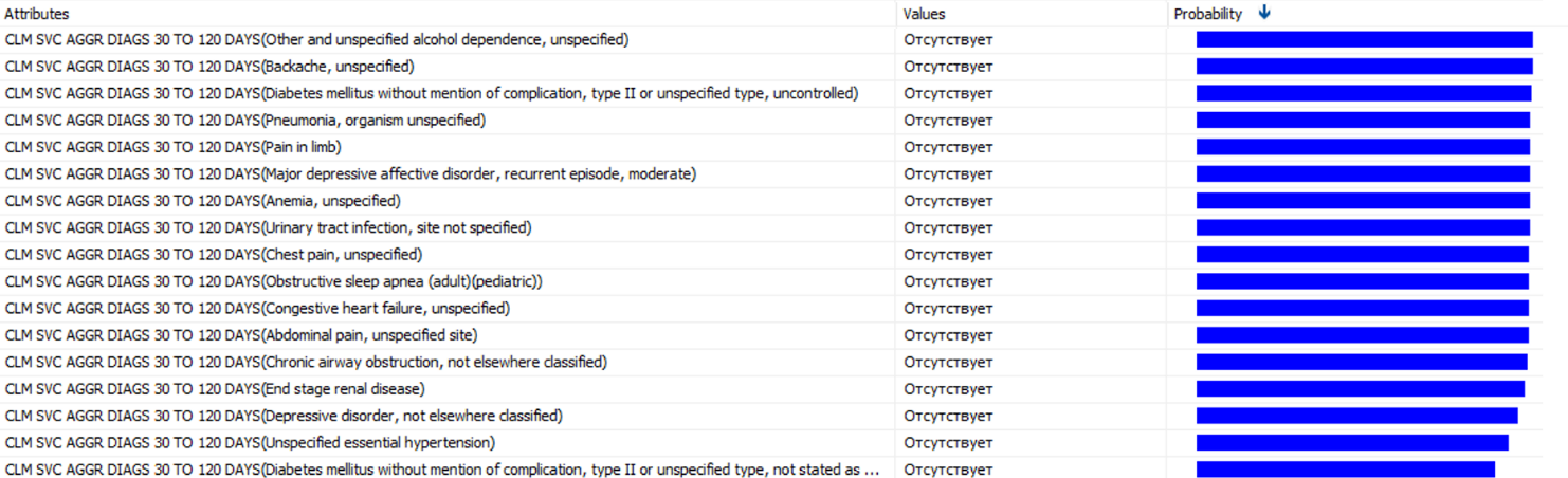
You can get a list of diagnoses, which most often precede large spending.
This is only part of the selected diagnoses. In each of the diagnoses, with a probability of from 85% to 100%, there will be a peak in costs. Their presence is worth making a separate sign. Do not miss the presence of conventional diagnoses, which will not cost the company expensive. Therefore, we should normalize the probabilities found and introduce a new sign, which will be a weighted sum of the number of diagnoses over the past 90 days.
As a result, seven parameters were obtained in the input feature vector. Compare them with what was obtained last time using different algorithms.
Testing various algorithms and setting their parameters
We will determine the parameters that will be used for training. Consider several different classification algorithms: logistic regression, support vector machine, decision jungle / random forest, Bayesian network. Neural networks are also an obvious option, but this is a separate complex topic and in this case this algorithm will be redundant.
Since the data was filtered to obtain a balanced sample, we will not change the boundary value for the assignment of classes. We will return to this question in the next article.
Logistic regression
This is a special case of a linear regressor adapted to the tasks of classification. The algorithm was already mentioned in the first article, where it was used to build the simplest model as a prototype.
At the initial stage, it allows you to get the initial value in the range from minus to plus infinity. Next, we perform the transformation using a sigmoid function of the form 1 / (1 + e ^ (- score)), where score is the value obtained earlier, we perform the conversion. The result will be a number ranging from -1 to +1. The decision to belong to the class is made on the basis of the selected threshold value.
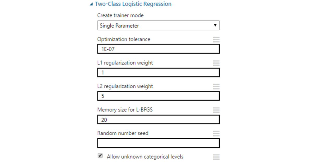
Options:
- Optimization tolerance - the limit for the minimum change in accuracy. If the difference between iterations becomes less than the specified value, learning stops. In most cases, you can leave the default value of 1E-7.
- L1 & L2 regularization - regularization according to the norms of order 1 and 2. L1 is used to reduce the dimension of the input data by removing the attributes that have the least effect on the result. L2 “finishes” signs with large coefficients, reducing these coefficients to zero at infinity. These values are coefficients for norms and, for starters, can remain equal to 1 by default.
- L-BFGS is an optimization method for finding the local maximum (minimum) of a non-linear functional without restrictions with limited memory. This is a quasi-Newtonian method (based on the accumulation of information about the curvature of the objective function for changing its gradient), used to weigh the parameters of the model. Here the choice depends on the preferences: the value set affects the amount of data used to invert the hessian function. Essentially, the specified number of last vectors is taken. Increasing this value improves accuracy. Improves to certain limits (do not forget about retraining). It can greatly increase the execution time, so it is often set in the vicinity of 10.
- Random seed can be set if necessary to obtain the same results on different runs of the algorithm.
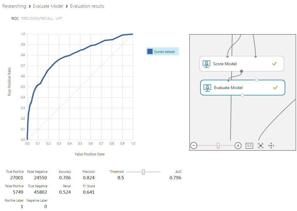
This algorithm was used in the prototype model, so the comparison will be most revealing. Even without adjusting the boundaries of the definition of classes and with small additions to the vector of input features, the percentage of correctly predicted peaks increased by 5%, and their absence increased by 15%. Such an important indicator, as the area under the curve of this graph, also increased significantly. This parameter reflects how well the values of classes relate to each other for different boundary values. The further the curve is from the diagonal, the better.
Support Vector Machine
The support vector method is included in the group of linear classifiers, although some modifications to the main part of the algorithm allow the construction of non-linear classifiers. The bottom line is to translate the source data into a higher dimension and build a separating hyperplane. Increasing the dimensionality is necessary, since the source vectors are often linearly inseparable. After translation, the hyperplane is searched for with the condition of maximum clearance to hyperplanes, denoting the boundary of classes.
Options:
- Number of iterations - the number of iterations of the learning algorithm. Represents a parameter for the exchange of accuracy and speed of the algorithm. For a start, you can put a value in the range from 1 to 10.
- Lambda - weight analogue for L1 in logistic regression
- Normalize features - normalize data before training. Due to the specifics of the method, in most cases the parameter should be left on by default.
- Project to unit sphere - normalization of coefficients. This parameter is optional and most often its use will not be needed.
- Allow unknown category - the default enabled parameter that allows the handling of unknown parameters of the model. It degrades the work of the model with those data that are known to the classifier, and at the same time improves the accuracy for unknowns.
- Random seed - similar to logistic regression.
The graph shows that this is not the most successful algorithm for this task. Accuracy and area under the curve are low. In addition, the curve itself is unstable in nature, which might be acceptable for the prototype, but not for the model with the processed data.
Bayesian network
Bayesian networks are a probabilistic data model, represented as an acyclic directed graph. The vertices of the graph are variables that reflect the truth of a certain judgment, and the edges are the degree of dependence between them. Setting up the model is the selection of these variables and the relationship between them. In our case, the final assessed judgment on which the graph converges will be the presence of a peak of costs.
Options:
- Number of training iterations - the same as the parameter in SVM.
- Include bias - the introduction of a constant value in the input parameters of the model. This is necessary when it is not in the source vector.
- Allow unknown values - similar to the parameter in SVM.
The Bayesian classifier showed results very similar to the results of logistic regression. Since the regression is simpler, we’ll dwell on it between them.
Random forest
This method is a committee of classic decision trees. In this algorithm, trees are not pruned (pruning is a method of reducing the complexity of a model through cutting branches of a tree after it is completely built). However, early stop conditions remain. Diversity is achieved by choosing random subsets of the source data. The size remains the same, but reuse of the same data is allowed in these subsets.
Each tree uses a random subset of attributes of size m (m is a tunable parameter, however, it is often suggested to use a value close to the root of the size of the original feature vector). The classification goes through a vote. The class with the most votes wins.
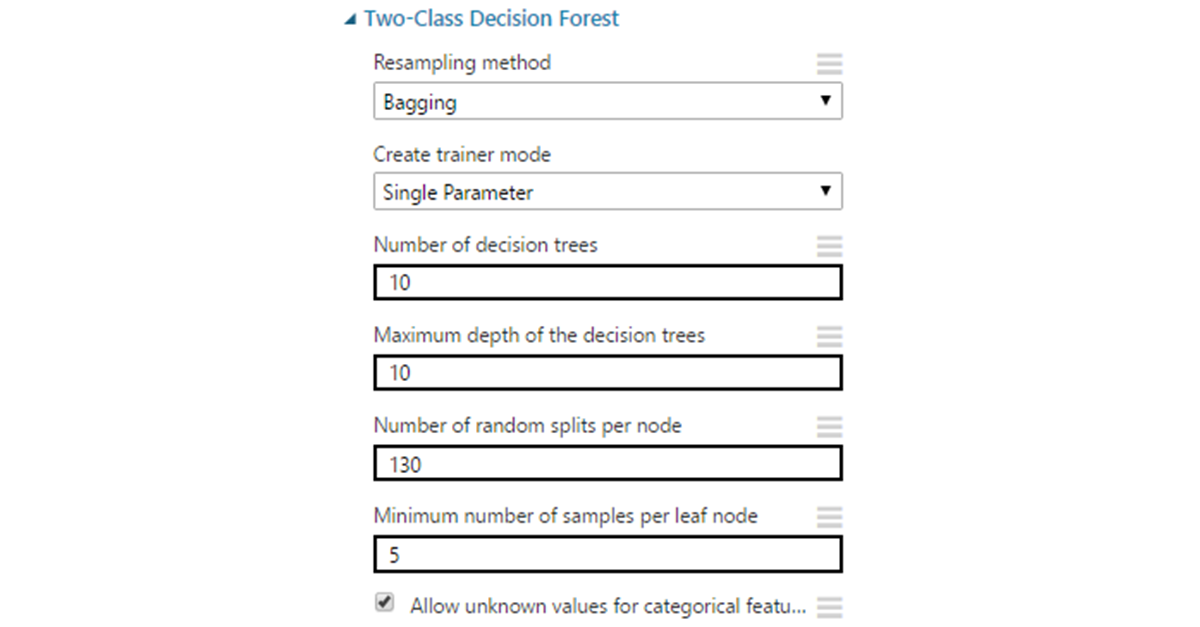
Options:
- The default resampling method is bagging, which gives each tree a unique selection of data as described above. You can also set replicate, if you need to train all trees on the same data.
- Number of decision trees . Increasing the number of trees can provide more sample coverage, but not always, and at the cost of increased training time.
- Maximum depth - the maximum depth of the tree. The default value - 32 - is quite large and in many situations will lead to retraining. Most often there is no need to do a depth of more than ten.
- Number of random splits per node - determines the number of random separation of signs when constructing vertices. Too much can lead to retraining, so it’s worth starting to limit to a value between 10 and 30.
- Minimum number of samples per leaf node - the minimum number of records for the formation of a "sheet" (vertices that are no longer subject to division into branches). It almost never makes sense to leave one in this place, since such leaves are redundant and often lead the model to retraining.
- Allow unknown values - similar to SVM.
Random forest turned out to be the most efficient algorithm, giving an increase in the definition of peaks by 8% and their absence by 13%. Important in the context of the problem is the best interpretability of the reasons for determining the data to any of the classes. Of course, this algorithm as a whole is a black box, but for it there are relatively simple ways to extract the necessary information.
In all the algorithms described above, except for Bayesian networks, there is a “create trainer mode” parameter. Putting it on the Parameter Range, you can enable the mode in which the algorithm learns on various options for the combination of parameters within the specified ranges, and gives the best option. This feature will illuminate later.
Using cross-validation to test variance
Cross-validation assessment can be used to solve various problems. For example, it is used to combat retraining in a small amount of data to isolate a separate validation sample. Now it will be required as a tool to test the ability of the current model to generalize. To do this, divide the data into ten parts and consider each of them as a test. Next, you will need to train the model on each version of the separation.
Take the algorithm that showed the best results among the others - Random Forest.
For all samples, the result is stable and quite high. The model has a good ability to generalize, and a sufficient amount of data is fed to the training.
Total
In this part of the series of articles on machine learning, we examined:
- Embedding Python scripts in the overall project scheme on the example of obtaining a data sample balanced by classes.
- Use MS Analysis Services to extract new traits from raw data.
- Cross-validation of the model to assess the stability of the result and completeness of data in the training set.
The results show a clear improvement in the accuracy and stability of the model. In the final article, we will address issues of retraining, statistical emissions and committees.
About the authors
The WaveAccess team creates technically complex, high-load and fault-tolerant software for companies from different countries. Commentary by Alexander Azarov, Head of Machine Learning at WaveAccess:
Machine learning allows you to automate areas where expert opinions currently dominate. This makes it possible to reduce the influence of the human factor and increase the scalability of the business.
Source: https://habr.com/ru/post/331484/
All Articles