Autoencoders in Keras, Part 1: Introduction

Content

• Part 1: Introduction
  
• Part 2: Manifold learning and latent variables
  
• Part 3: Variational autoencoders ( VAE )
  
• Part 4: Conditional VAE
  
• Part 5: GAN (Generative Adversarial Networks) and tensorflow
  
• Part 6: VAE + GAN
  

While diving into Deep Learning, the topic of auto-encoders caught me, especially in terms of generating new objects. In an effort to improve the quality of generation, read various blogs and literature on the topic of generative approaches. As a result, the accumulated experience decided to clothe in a small series of articles, in which he tried briefly and with examples to describe all those problem areas he had encountered himself, at the same time introducing Keras into the syntax.

Autoencoders

Autoencoders are direct propagation neural networks that regenerate the input signal at the output. Inside they have a hidden layer, which is the code that describes the model. Autoencoders are designed in such a way as to not be able to accurately copy the input to the output. Usually they are limited in the dimension of the code (it is less than the dimension of the signal) or fined for activation in the code . The input signal is recovered with errors due to coding losses, but in order to minimize them, the network has to learn to select the most important features.


')
Who cares, welcome under the cat


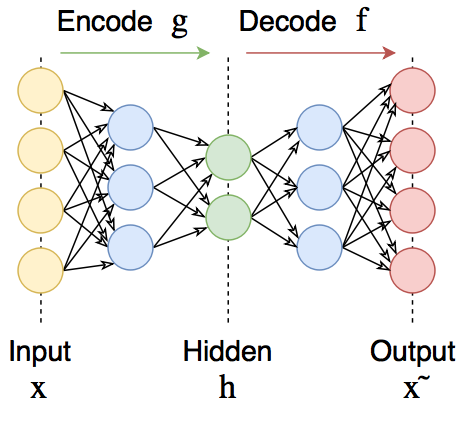
Autoencoders consist of two parts: encoder and decoder . The encoder translates the input signal into its presentation ( code ): and the decoder recovers the signal by its code : .

Autoencoder changing and seeking to learn the identity function minimizing some kind of error functional.


Moreover, the family of encoder functions and decoder somehow limited to autoencoder was forced to select the most important properties of the signal.

The ability of autoencoders to compress data itself is rarely used, as they usually work worse than hand-written algorithms for specific data types like sounds or images. It is also critically important for them that the data belong to the general population on which the network was trained. Having trained the autoencoder on numbers, it cannot be used to encode something else (for example, human faces).

However, autoencoders can be used for pre-training, for example, when there is a classification task, and there are too few marked pairs. Or to reduce the dimension in the data for later visualization. Or when you just need to learn to distinguish between the useful properties of the input signal.

Moreover, some of their developments (which will also be described later), such as variational autoencoder ( VAE ), as well as its combination with competing generative networks ( GAN ), give very interesting results and are now at the forefront of the science of generative models.

Keras

Keras is a very convenient high-level library for deep learning, working on top of theano or tensorflow . It is based on layers, connecting them together, we get the model. Once created, the models and layers retain their internal parameters, and therefore, for example, you can train a layer in one model and use it in another, which is very convenient.

Keras models are easy to save / load, they have a simple, but at the same time deeply customizable learning process; models are freely embedded in the tensorflow / theano code (as operations on tensors).

We will use dataset of handwritten numbers MNIST as data.

Download it:

from keras.datasets import mnist import numpy as np (x_train, y_train), (x_test, y_test) = mnist.load_data() x_train = x_train.astype('float32') / 255. x_test = x_test .astype('float32') / 255. x_train = np.reshape(x_train, (len(x_train), 28, 28, 1)) x_test = np.reshape(x_test, (len(x_test), 28, 28, 1)) 

Compression autoencoder

To begin with, we will create the simplest (compressing, undercomplete) autoencoder with a small-dimension code of two fully connected layers: an encoder and a decoder.

Since the intensity of the color is normalized to unity, then we take sigmoid activation of the output layer.

Let's write separate models for the encoder, decoder and the whole autoencoder. To do this, create instances of the layers and apply them one by one, finally combining everything into models.

 from keras.layers import Input, Dense, Flatten, Reshape from keras.models import Model def create_dense_ae(): #    encoding_dim = 49 #  #   input_img = Input(shape=(28, 28, 1)) # 28, 28, 1 -  , ,   ,  - #    flat_img = Flatten()(input_img) #     encoded = Dense(encoding_dim, activation='relu')(flat_img) #  #      input_encoded = Input(shape=(encoding_dim,)) flat_decoded = Dense(28*28, activation='sigmoid')(input_encoded) decoded = Reshape((28, 28, 1))(flat_decoded) # ,       ,     #          encoder = Model(input_img, encoded, name="encoder") decoder = Model(input_encoded, decoded, name="decoder") autoencoder = Model(input_img, decoder(encoder(input_img)), name="autoencoder") return encoder, decoder, autoencoder 

Create and compile the model (compilation in this case refers to the construction of the graph of calculations for back propagation of error )

 encoder, decoder, autoencoder = create_dense_ae() autoencoder.compile(optimizer='adam', loss='binary_crossentropy') 

Look at the number of parameters

 autoencoder.summary() 

 _________________________________________________________________ Layer (type) Output Shape Param # ================================================================= input_1 (InputLayer) (None, 28, 28, 1) 0 _________________________________________________________________ encoder (Model) (None, 49) 38465 _________________________________________________________________ decoder (Model) (None, 28, 28, 1) 39200 ================================================================= Total params: 77,665.0 Trainable params: 77,665.0 Non-trainable params: 0.0 _________________________________________________________________ 

Now we will train our autoencoder

 autoencoder.fit(x_train, x_train, epochs=50, batch_size=256, shuffle=True, validation_data=(x_test, x_test)) 

 Epoch 46/50 60000/60000 [==============================] - 3s - loss: 0.0785 - val_loss: 0.0777 Epoch 47/50 60000/60000 [==============================] - 2s - loss: 0.0784 - val_loss: 0.0777 Epoch 48/50 60000/60000 [==============================] - 3s - loss: 0.0784 - val_loss: 0.0777 Epoch 49/50 60000/60000 [==============================] - 2s - loss: 0.0784 - val_loss: 0.0777 Epoch 50/50 60000/60000 [==============================] - 3s - loss: 0.0784 - val_loss: 0.0777 

Digit drawing function

 %matplotlib inline import seaborn as sns import matplotlib.pyplot as plt def plot_digits(*args): args = [x.squeeze() for x in args] n = min([x.shape[0] for x in args]) plt.figure(figsize=(2*n, 2*len(args))) for j in range(n): for i in range(len(args)): ax = plt.subplot(len(args), n, i*n + j + 1) plt.imshow(args[i][j]) plt.gray() ax.get_xaxis().set_visible(False) ax.get_yaxis().set_visible(False) plt.show() 

Encode several images and, for the sake of interest, take a look at the sample code.

 n = 10 imgs = x_test[:n] encoded_imgs = encoder.predict(imgs, batch_size=n) encoded_imgs[0] 

 array([ 6.64665604, 7.53528595, 3.81508064, 4.66803837, 1.50886345, 5.41063929, 9.28293324, 10.79530716, 0.39599913, 4.20529413, 6.53982353, 5.64758158, 5.25313473, 1.37336707, 9.37590599, 6.00672245, 4.39552879, 5.39900637, 4.11449528, 7.490417 , 10.89267063, 7.74325705, 13.35806847, 3.59005809, 9.75185394, 2.87570286, 3.64097357, 7.86691713, 5.93383646, 5.52847338, 3.45317888, 1.88125253, 7.471385 , 7.29820824, 10.02830505, 10.5430584 , 3.2561543 , 8.24713707, 2.2687614 , 6.60069561, 7.58116722, 4.48140812, 6.13670635, 2.9162209 , 8.05503941, 10.78182602, 4.26916027, 5.17175484, 6.18108797], dtype=float32) 

We decode these codes and compare them with the originals.

 decoded_imgs = decoder.predict(encoded_imgs, batch_size=n) plot_digits(imgs, decoded_imgs) 

Deep autoencoder

No one bothers us to make the same autoencoder, but with a large number of layers. In this case, he will be able to isolate more complex nonlinear patterns

 def create_deep_dense_ae(): #    encoding_dim = 49 #  input_img = Input(shape=(28, 28, 1)) flat_img = Flatten()(input_img) x = Dense(encoding_dim*3, activation='relu')(flat_img) x = Dense(encoding_dim*2, activation='relu')(x) encoded = Dense(encoding_dim, activation='linear')(x) #  input_encoded = Input(shape=(encoding_dim,)) x = Dense(encoding_dim*2, activation='relu')(input_encoded) x = Dense(encoding_dim*3, activation='relu')(x) flat_decoded = Dense(28*28, activation='sigmoid')(x) decoded = Reshape((28, 28, 1))(flat_decoded) #  encoder = Model(input_img, encoded, name="encoder") decoder = Model(input_encoded, decoded, name="decoder") autoencoder = Model(input_img, decoder(encoder(input_img)), name="autoencoder") return encoder, decoder, autoencoder d_encoder, d_decoder, d_autoencoder = create_deep_dense_ae() d_autoencoder.compile(optimizer='adam', loss='binary_crossentropy') 

Look at the summary of our model

 d_autoencoder.summary() 

 _________________________________________________________________ Layer (type) Output Shape Param # ================================================================= input_3 (InputLayer) (None, 28, 28, 1) 0 _________________________________________________________________ encoder (Model) (None, 49) 134750 _________________________________________________________________ decoder (Model) (None, 28, 28, 1) 135485 ================================================================= Total params: 270,235.0 Trainable params: 270,235.0 Non-trainable params: 0.0 

The number of parameters has grown more than 3 times, let's see if the new model will cope better:

 d_autoencoder.fit(x_train, x_train, epochs=100, batch_size=256, shuffle=True, validation_data=(x_test, x_test)) 

 Epoch 96/100 60000/60000 [==============================] - 3s - loss: 0.0722 - val_loss: 0.0724 Epoch 97/100 60000/60000 [==============================] - 3s - loss: 0.0722 - val_loss: 0.0719 Epoch 98/100 60000/60000 [==============================] - 3s - loss: 0.0721 - val_loss: 0.0722 Epoch 99/100 60000/60000 [==============================] - 3s - loss: 0.0721 - val_loss: 0.0720 Epoch 100/100 60000/60000 [==============================] - 3s - loss: 0.0721 - val_loss: 0.0720 

 n = 10 imgs = x_test[:n] encoded_imgs = d_encoder.predict(imgs, batch_size=n) encoded_imgs[0] decoded_imgs = d_decoder.predict(encoded_imgs, batch_size=n) plot_digits(imgs, decoded_imgs) 

We see that the loss is saturated at a much lower value, and the numbers are a bit more pleasant.

Convolution autoencoder

Since we work with pictures, there must be some spatial invariance in the data. Let's try to use this: let's build a convolutional autoencoder

 from keras.layers import Conv2D, MaxPooling2D, UpSampling2D def create_deep_conv_ae(): input_img = Input(shape=(28, 28, 1)) x = Conv2D(128, (7, 7), activation='relu', padding='same')(input_img) x = MaxPooling2D((2, 2), padding='same')(x) x = Conv2D(32, (2, 2), activation='relu', padding='same')(x) x = MaxPooling2D((2, 2), padding='same')(x) encoded = Conv2D(1, (7, 7), activation='relu', padding='same')(x) #     (7, 7, 1) .. 49- input_encoded = Input(shape=(7, 7, 1)) x = Conv2D(32, (7, 7), activation='relu', padding='same')(input_encoded) x = UpSampling2D((2, 2))(x) x = Conv2D(128, (2, 2), activation='relu', padding='same')(x) x = UpSampling2D((2, 2))(x) decoded = Conv2D(1, (7, 7), activation='sigmoid', padding='same')(x) #  encoder = Model(input_img, encoded, name="encoder") decoder = Model(input_encoded, decoded, name="decoder") autoencoder = Model(input_img, decoder(encoder(input_img)), name="autoencoder") return encoder, decoder, autoencoder c_encoder, c_decoder, c_autoencoder = create_deep_conv_ae() c_autoencoder.compile(optimizer='adam', loss='binary_crossentropy') c_autoencoder.summary() 

 _________________________________________________________________ Layer (type) Output Shape Param # ================================================================= input_5 (InputLayer) (None, 28, 28, 1) 0 _________________________________________________________________ encoder (Model) (None, 7, 7, 1) 24385 _________________________________________________________________ decoder (Model) (None, 28, 28, 1) 24385 ================================================================= Total params: 48,770.0 Trainable params: 48,770.0 Non-trainable params: 0.0 

 c_autoencoder.fit(x_train, x_train, epochs=64, batch_size=256, shuffle=True, validation_data=(x_test, x_test)) 

 Epoch 60/64 60000/60000 [==============================] - 24s - loss: 0.0698 - val_loss: 0.0695 Epoch 61/64 60000/60000 [==============================] - 24s - loss: 0.0699 - val_loss: 0.0705 Epoch 62/64 60000/60000 [==============================] - 24s - loss: 0.0699 - val_loss: 0.0694 Epoch 63/64 60000/60000 [==============================] - 24s - loss: 0.0698 - val_loss: 0.0691 Epoch 64/64 60000/60000 [==============================] - 24s - loss: 0.0697 - val_loss: 0.0693 

 n = 10 imgs = x_test[:n] encoded_imgs = c_encoder.predict(imgs, batch_size=n) decoded_imgs = c_decoder.predict(encoded_imgs, batch_size=n) plot_digits(imgs, decoded_imgs) 

Despite the fact that the number of parameters of this network is much less than that of fully connected networks, the error function is saturated at a much smaller value.

Denoising autoencoder

Autoencoders can be trained to remove noise from the data: to do this, it is necessary to input noisy data at the output and compare it with the data without noise:


Where - noisy data.

In Keras, you can wrap arbitrary operations from the underlying framework into the Lambda layer. You can access operations from tensorflow or theano through the backend module.

Let's create a model that will noise the input image, and relieve any noise by retraining any of the already created autoencoders.

 import keras.backend as K from keras.layers import Lambda batch_size = 16 def create_denoising_model(autoencoder): def add_noise(x): noise_factor = 0.5 x = x + K.random_normal(x.get_shape(), 0.5, noise_factor) x = K.clip(x, 0., 1.) return x input_img = Input(batch_shape=(batch_size, 28, 28, 1)) noised_img = Lambda(add_noise)(input_img) noiser = Model(input_img, noised_img, name="noiser") denoiser_model = Model(input_img, autoencoder(noiser(input_img)), name="denoiser") return noiser, denoiser_model noiser, denoiser_model = create_denoising_model(autoencoder) denoiser_model.compile(optimizer='adam', loss='binary_crossentropy') 

 denoiser_model.fit(x_train, x_train, epochs=200, batch_size=batch_size, shuffle=True, validation_data=(x_test, x_test)) 

 n = 10 imgs = x_test[:batch_size] noised_imgs = noiser.predict(imgs, batch_size=batch_size) encoded_imgs = encoder.predict(noised_imgs[:n], batch_size=n) decoded_imgs = decoder.predict(encoded_imgs[:n], batch_size=n) plot_digits(imgs[:n], noised_imgs, decoded_imgs) 

The numbers on noisy images are hard to see , but the denoising autoencoder removed the noise quite well and the numbers became quite readable.

Sparse autoencoder

A sparse autoencoder is simply an autoencoder whose penalty is added to the loss function for the values ​​in the code , that is, the autoencoder seeks to minimize such an error function:


Where - code,

- the usual regularizer (for example, L1):


Sparse autoencoder does not necessarily taper to the center. Its code may have a higher dimension than the input signal. Learning to approximate the identical function , he learns in the code to highlight the useful properties of the signal. Because of the regularizer, even a sparse autoencoder expanding towards the center cannot learn the identical function directly.

 from keras.regularizers import L1L2 def create_sparse_ae(): encoding_dim = 16 lambda_l1 = 0.00001 #  input_img = Input(shape=(28, 28, 1)) flat_img = Flatten()(input_img) x = Dense(encoding_dim*3, activation='relu')(flat_img) x = Dense(encoding_dim*2, activation='relu')(x) encoded = Dense(encoding_dim, activation='linear', activity_regularizer=L1L2(lambda_l1))(x) #  input_encoded = Input(shape=(encoding_dim,)) x = Dense(encoding_dim*2, activation='relu')(input_encoded) x = Dense(encoding_dim*3, activation='relu')(x) flat_decoded = Dense(28*28, activation='sigmoid')(x) decoded = Reshape((28, 28, 1))(flat_decoded) #  encoder = Model(input_img, encoded, name="encoder") decoder = Model(input_encoded, decoded, name="decoder") autoencoder = Model(input_img, decoder(encoder(input_img)), name="autoencoder") return encoder, decoder, autoencoder s_encoder, s_decoder, s_autoencoder = create_sparse_ae() s_autoencoder.compile(optimizer='adam', loss='binary_crossentropy') 

 s_autoencoder.fit(x_train, x_train, epochs=400, batch_size=256, shuffle=True, validation_data=(x_test, x_test)) 

Look at the codes

 n = 10 imgs = x_test[:n] encoded_imgs = s_encoder.predict(imgs, batch_size=n) encoded_imgs[1] 

 array([ 7.13531828, -0.61532277, -5.95510817, 12.0058918 , -1.29253936, -8.56000137, -7.48944521, -0.05415952, -2.81205249, -8.4289856 , -0.67815018, -11.19531345, -3.4353714 , 3.18580866, -0.21041733, 4.13229799], dtype=float32) 

 decoded_imgs = s_decoder.predict(encoded_imgs, batch_size=n) plot_digits(imgs, decoded_imgs) 

Let's see if we can somehow interpret the dimensions in codes.
Take the average of all codes, and then in turn each dimension in the averaged code is replaced by its maximum value.

 imgs = x_test encoded_imgs = s_encoder.predict(imgs, batch_size=16) codes = np.vstack([encoded_imgs.mean(axis=0)]*10) np.fill_diagonal(codes, encoded_imgs.max(axis=0)) decoded_features = s_decoder.predict(codes, batch_size=16) plot_digits(decoded_features) 

Some features look, but nothing sensible here is not visible.

The values ​​in the codes one by one do not carry any obvious meaning, only the cunning interaction between the values ​​that occurs in the layers of the decoder allows it to restore the input signal by code.

Is it possible to generate objects from codes at will?

In order to answer this question, it is better to study what codes are and how they can be interpreted. About this in the next part .

Useful links and literature

This post is based on our own interpretation of the first part of the post of the creator Keras Francois Chollet about autoencoders in Keras .

As well as chapters about autoencoders in the Deep Learning Book .