Useful features of Google Spreadsheet that are not in Excel
The article is written in collaboration with Renat Shagabutdinov.

This article will discuss some very useful features of Google Spreadsheets that are not in Excel (SORT, array combining, FILTER, IMPORTRANGE, IMAGE, GOOGLETRANSLATE, DETECTLANGUAGE)
')
There are a lot of letters, but there are interesting case studies, all the examples, by the way, can be viewed closer in the Google Document goo.gl/cOQAd9 ( file- > create a copy to copy the file to Google Drive and be editable).
Table of contents:
- If the result of a formula is multiple cells
- Combining multiple data ranges for use in formulas
- SORT
- How to add table headers in SORT?
- FILTER
- FILTER, two conditions and work with date
- Interactive Graphic with FILTER and SPARKLINE
- IMPORTRANGE
- Import formatting from source table
- IMPORTRANGE as an argument to another function.
- IMAGE: add images to cells
- GOOGLETRANSLATE and DETECTLANGUAGE: translate text in cells
If the result of a formula takes more than one cell
First, an important feature of displaying the results of formulas in Google Spreadsheets. If your formula returns more than one cell, then this entire array will be displayed immediately and take as many cells and columns as you need for it (in Excel, you would need to enter the array formula in all these cells). In the following example, let's see how it works.
It will help to sort the data range by one or several columns and display the result immediately.
Function syntax:
The example in the screenshot below, we entered the formula only in cell D2 and sorted the data by the first column (instead of TRUE / FALSE, you can enter TRUE / FALSE).

How to add table headers in SORT?
Using curly brackets {} we create an array of two elements, the caps of table A1: B1 and the function SORT, separate the elements from each other using a semicolon.
How to combine multiple data ranges and sort (and not only)?
Let's look at how you can combine ranges for use in functions. This applies not only to SORT, this technique can be used in any function, where it is possible, for example, in CDF or MATCH.
Someone who has read the previous example has already figured out what to do: open the curly bracket and collect arrays to join, separating them from each other with a semicolon and closing the curly bracket.

You can combine arrays and not use them in a formula, but simply output to a sheet, say, by collecting data from several sheets of your book. For vertical merging, it is necessary to observe only the same number of columns in all fragments (we have two columns everywhere).

And in the screenshot below - an example of horizontal union, instead of a semicolon, a backslash is used in it and it is necessary that the number of lines in the fragments match, otherwise the formula will return an error instead of a combined range.
Now let's go back to the horizontal array and insert it into the SORT function. We will sort the data by the first column in descending order.
Merging can be used in any functions, the main thing is to observe the same number of columns for vertical or rows for horizontal merging.
All analyzed examples can be viewed closer.
Google Document .
Using FILTER, we can filter data by one or several conditions and display the result on a worksheet or use the result in another function, like a data range.
Function syntax:
One condition
Example, we have a table with sales of our employees, we derive data from it on one employee.
Let's enter into the cell E3 the following formula:
Note that the syntax is slightly different from the usual formulas, like SUMMESLIN, where the range of the condition and the condition itself would be separated with a semicolon.
The formula entered in one cell returns us an array of 9 cells with data, but after examples with the SORT function, we are no longer surprised.
In addition to the equal sign (=) in the conditions, you can also use>,> =, <> (not equal), <, <=. For textual conditions, only = and <> are suitable, and for numbers or dates, all of these characters can be used.
Two conditions and work with date
Let's complicate the formula and add one more condition to it, according to the sales date, leave all sales starting from 01.02.17
This is how the formula will look like, if you enter the condition arguments immediately into it, pay attention to converting the text entry of the date using DATEVALUE:
Or like this, if you refer to cells with arguments:
Interactive Graphic with FILTER and SPARKLINE
Do you know how else you can use the FILTER function? We can not display the result of a function on a worksheet, but use it as data for another function, for example, a sparkline. Sparkline is a function that builds a graph in a cell based on our data, there are many settings in the sparkline, such as the type of graph, the color of the elements, but now we will not dwell on them and use the function without additional settings. Let's move on to an example.
Drop-down list. Our schedule will change depending on the selected employee in the drop-down list, the list is done like this:
Click "Save" and get a drop-down list in the selected cell:

A cell with a drop-down list will become a condition for the FILTER formula, we will write it.
And we will insert this formula into the SPARKLINE function, which will draw a graph in the cell based on the data obtained.

So it looks in dynamics:
And here’s how a SPARKLINE can look elegant with additional settings, in real work, the diagram displays the results of activities in one day, the green columns show positive values, and the pink ones show negative values.
To transfer data from one file to another, Google Spreadsheets uses the IMPORTRANGE function.
When can it be useful?
This formula allows you to get a copy of the range from another Google spreadsheet. The formatting is not transferred - only the data (how to deal with the formatting - we will tell a little below).
The formula syntax is as follows:
spreadsheet_key (key) - the sequence of characters of the “key =” attribute (key) in the link to the table (after “spreadsheets / ... /”).
Example of a formula with a key:
Instead of a table key, you can use the full link to the document:
Your file will display the range A1: CM500 from Sheet1 from the file that is located on the corresponding link.
If the number of columns or rows in the source file may change, enter the open range in the second argument of the function (see also subsection “A2: A type ranges”), for example:
! Keep in mind that if you load an open range (for example, A1: D), then you will not be able to insert any data manually into columns A: D in the file where the IMPORTRANGE formula is located (that is, at the end where the data is loaded). They seem to be “reserved” for the entire open range - because its dimension is unknown in advance.
The link to the file and the link to the range can be entered not into the formula, but into the cells of your document and refer to them.
So, if in cell A1 you enter a link to a document (without quotes) from which you want to load data, and in cell B1 you can enter a link to a sheet and a range (also without quotes), then you can import data using the following formula:

The option with links to cells is preferable in the sense that you can always easily go to the source file (by clicking the link in the cell) and / or see which range and which tab is being imported.
As we have already noted, IMPORTRANGE loads only data, but not the formatting of the source table. How to deal with this? Prepare the soil in advance by copying the formatting from the source sheet. To do this, go to the source sheet and copy it into your book:
After clicking the Copy to ... button, select the book into which you will import data. Usually the table you need is on the Recent tab (if you’ve really recently worked with it).
After copying the sheet, select all the data (by clicking on the upper left corner):
And click Delete . All data will disappear, but the formatting will remain. Now you can enter the IMPORTRANGE function and get a full match of the source sheet - both in the data part and in the format part:
IMPORTRANGE as an argument to another function.
IMPORTRANGE can be an argument to another function if the range you are importing is suitable for this role.
Consider a simple example - the average value of sales from a range that is in another document.
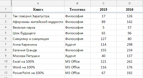
This is the original document. Let the data be added and we need the 2016 average of sales (that is, from cell D2 and all the way down).
First we import this range:
And then use this as an argument of the AVERAGE function:
We get the result, which will be updated when adding new lines in the source file in column D.
The IMAGE feature allows you to add images to your Google Spreadsheets cells.
The function has the following syntax:
URL is the only required argument. This is a link to the image. The link can be specified directly in the formula, taking in quotes:
Or put a link to the cell in which the link is stored:
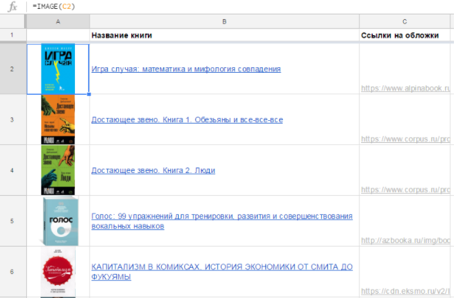
The latter option is more convenient in most cases. So, if you have a list of books and links to covers, one formula is enough to display them all:
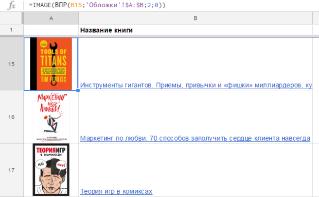
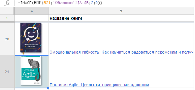
In practice, it happens that links to images are stored on a separate sheet, and you get them using the VLOOKUP function or something else.
The mode argument can take four values (if you omit it, the first will be the default):
Let's see how images look in practice with four different values of the mode argument:

The fourth mode can be convenient if you need to select the exact image size in pixels by changing the height and width parameters. The picture will be immediately updated.
Note that for all modes except the second, there may be empty areas in the cell, and they can be filled with color:
In Google Spreadsheets, there is an interesting function GOOGLETRANSLATE, which allows you to translate text directly into cells:

The syntax of the function is as follows:
text is the text to be translated. You can take the text in quotes and write directly into the formula, but it is more convenient to refer to the cell in which the text is written.
[source_language] - the language from which we translate;
[target_language] is the language we translate into.
The second and third arguments are given by a two-digit code: es, fr, en, ru. They can also be specified in the function itself, but can be taken from the cell, and the source text language can be automatically determined.

And what if we want to translate into different languages? And at the same time we do not want to specify the source language manually every time?
This is where the DETECTLANGUAGE function comes in handy. It has a single argument — the text whose language is to be determined:
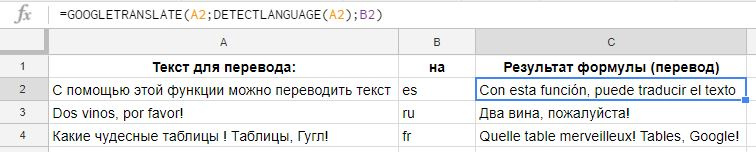
As with any other function, the beauty here is in automation. You can quickly change the text or language; quickly translate one phrase into 10 languages and so on. Of course, we understand that this is the text of the online translator - the quality will be appropriate.
Yevgeny Namokonov and Renat Shagabutdinov, and we also lead a channel in a telegram, where we analyze different cases with Google Spreadsheets, if you are interested, look in on a visit, you can find the link in my profile.
This article will discuss some very useful features of Google Spreadsheets that are not in Excel (SORT, array combining, FILTER, IMPORTRANGE, IMAGE, GOOGLETRANSLATE, DETECTLANGUAGE)
')
There are a lot of letters, but there are interesting case studies, all the examples, by the way, can be viewed closer in the Google Document goo.gl/cOQAd9 ( file- > create a copy to copy the file to Google Drive and be editable).
Table of contents:
- If the result of a formula is multiple cells
- Combining multiple data ranges for use in formulas
- SORT
- How to add table headers in SORT?
- FILTER
- FILTER, two conditions and work with date
- Interactive Graphic with FILTER and SPARKLINE
- IMPORTRANGE
- Import formatting from source table
- IMPORTRANGE as an argument to another function.
- IMAGE: add images to cells
- GOOGLETRANSLATE and DETECTLANGUAGE: translate text in cells
If the result of a formula takes more than one cell
First, an important feature of displaying the results of formulas in Google Spreadsheets. If your formula returns more than one cell, then this entire array will be displayed immediately and take as many cells and columns as you need for it (in Excel, you would need to enter the array formula in all these cells). In the following example, let's see how it works.
SORT
It will help to sort the data range by one or several columns and display the result immediately.
Function syntax:
= SORT (data to be sorted; column_for_sorting; increment; [column_for_sort_2, increment_2; ...])
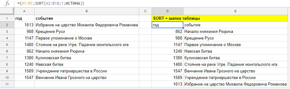
The example in the screenshot below, we entered the formula only in cell D2 and sorted the data by the first column (instead of TRUE / FALSE, you can enter TRUE / FALSE).
(hereinafter - examples for the Russian regional table settings, reg. settings are changed in the file menu → table settings)
How to add table headers in SORT?
Using curly brackets {} we create an array of two elements, the caps of table A1: B1 and the function SORT, separate the elements from each other using a semicolon.
How to combine multiple data ranges and sort (and not only)?
Let's look at how you can combine ranges for use in functions. This applies not only to SORT, this technique can be used in any function, where it is possible, for example, in CDF or MATCH.
Someone who has read the previous example has already figured out what to do: open the curly bracket and collect arrays to join, separating them from each other with a semicolon and closing the curly bracket.
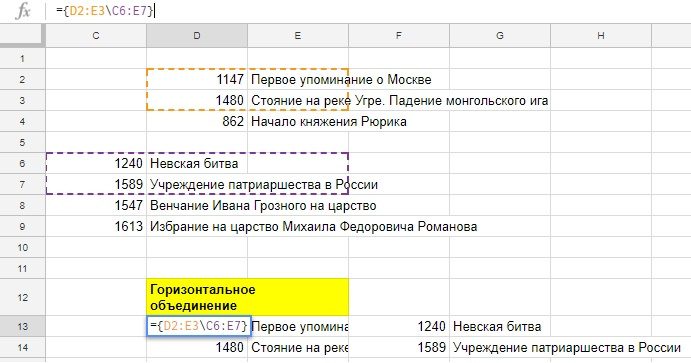
You can combine arrays and not use them in a formula, but simply output to a sheet, say, by collecting data from several sheets of your book. For vertical merging, it is necessary to observe only the same number of columns in all fragments (we have two columns everywhere).
And in the screenshot below - an example of horizontal union, instead of a semicolon, a backslash is used in it and it is necessary that the number of lines in the fragments match, otherwise the formula will return an error instead of a combined range.
(semicolon and backslash are the separators of the array elements in the Russian regional settings, if the examples do not work for you, then through the file - the table settings, make sure that they are you)
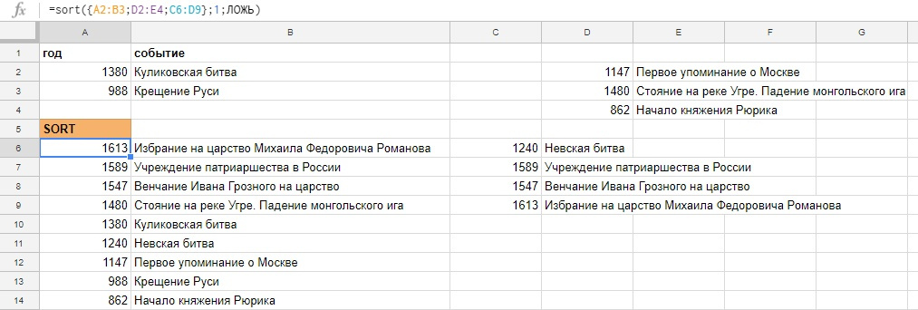
Now let's go back to the horizontal array and insert it into the SORT function. We will sort the data by the first column in descending order.
Merging can be used in any functions, the main thing is to observe the same number of columns for vertical or rows for horizontal merging.
All analyzed examples can be viewed closer.
Google Document .
Filter
Using FILTER, we can filter data by one or several conditions and display the result on a worksheet or use the result in another function, like a data range.
Function syntax:
FILTER (range; condition_1; [condition_2; ...])
One condition
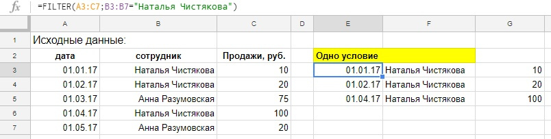
Example, we have a table with sales of our employees, we derive data from it on one employee.
Let's enter into the cell E3 the following formula:
= FILTER (A3: C7; B3: B7 = "Natalya Chistyakova")
Note that the syntax is slightly different from the usual formulas, like SUMMESLIN, where the range of the condition and the condition itself would be separated with a semicolon.
The formula entered in one cell returns us an array of 9 cells with data, but after examples with the SORT function, we are no longer surprised.
In addition to the equal sign (=) in the conditions, you can also use>,> =, <> (not equal), <, <=. For textual conditions, only = and <> are suitable, and for numbers or dates, all of these characters can be used.
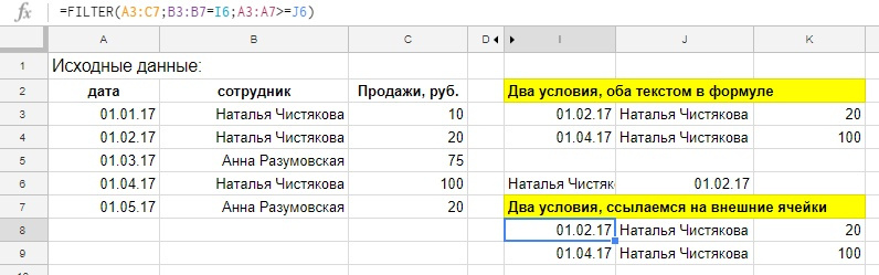
Two conditions and work with date
Let's complicate the formula and add one more condition to it, according to the sales date, leave all sales starting from 01.02.17
This is how the formula will look like, if you enter the condition arguments immediately into it, pay attention to converting the text entry of the date using DATEVALUE:
= FILTER (A3: C7; B3: B7 = "Natalia Chistyakova"; A3: A7> = DATENAME ("02.02.17"))
Or like this, if you refer to cells with arguments:
= FILTER (A3: C7; B3: B7 = I6; A3: A7> = J6)
Interactive Graphic with FILTER and SPARKLINE
Do you know how else you can use the FILTER function? We can not display the result of a function on a worksheet, but use it as data for another function, for example, a sparkline. Sparkline is a function that builds a graph in a cell based on our data, there are many settings in the sparkline, such as the type of graph, the color of the elements, but now we will not dwell on them and use the function without additional settings. Let's move on to an example.
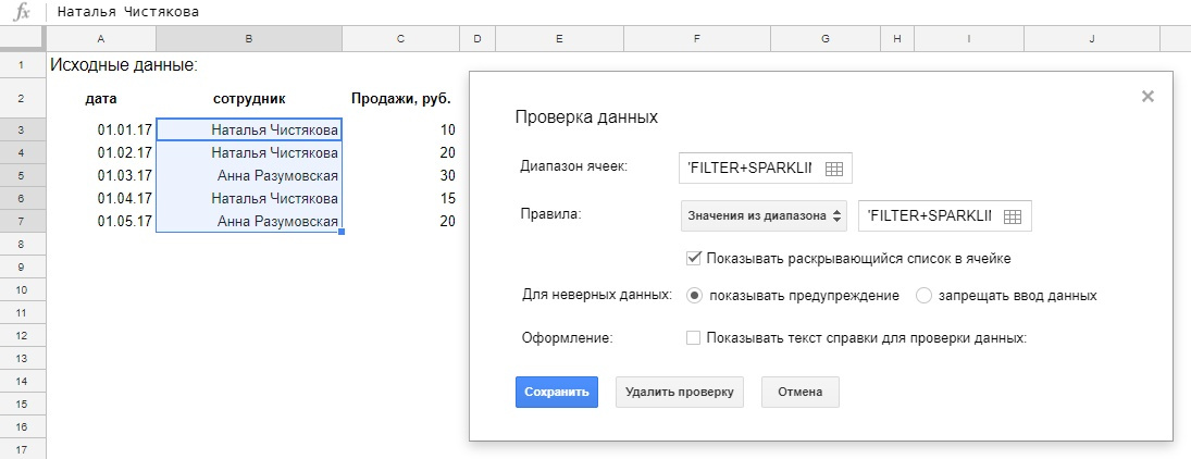
Drop-down list. Our schedule will change depending on the selected employee in the drop-down list, the list is done like this:
- select the E2 cell;
- Data menu → Data validation;
- rules: Value from a range and in a range; select a column with employees from the initial data; do not worry that the surnames are repeated, only unique values will remain in the drop-down list;
Click "Save" and get a drop-down list in the selected cell:
A cell with a drop-down list will become a condition for the FILTER formula, we will write it.
= FILTER (C3: C7; B3: B7 = E2)
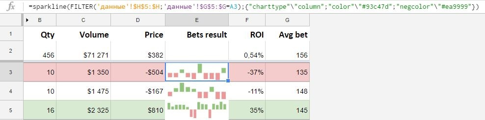
And we will insert this formula into the SPARKLINE function, which will draw a graph in the cell based on the data obtained.
= sparkline (FILTER (C3: C7; B3: B7 = E2))
So it looks in dynamics:
And here’s how a SPARKLINE can look elegant with additional settings, in real work, the diagram displays the results of activities in one day, the green columns show positive values, and the pink ones show negative values.
IMPORTRANGE
To transfer data from one file to another, Google Spreadsheets uses the IMPORTRANGE function.
When can it be useful?
- You need actual data from your colleagues file.
- You want to process data from a file to which you have “View Only” access.
- You want to collect tables from several documents in one place in order to process or view them.
This formula allows you to get a copy of the range from another Google spreadsheet. The formatting is not transferred - only the data (how to deal with the formatting - we will tell a little below).
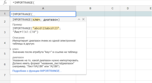
The formula syntax is as follows:
IMPORTRANGE (spreadsheet key; range string)
IMPORTRANGE (key; range)
spreadsheet_key (key) - the sequence of characters of the “key =” attribute (key) in the link to the table (after “spreadsheets / ... /”).
Example of a formula with a key:
= IMPORTRANGE ("abcd123abcd123"; "sheet1! A1: C10")
Instead of a table key, you can use the full link to the document:
= IMPORTRANGE (" docs.google.com/a/company_site.com/spreadsheet/ccc?key=0A601pBdE1zIzHRxcGZFVT3hyVyWc "; "Sheet1! A1: CM500")
Your file will display the range A1: CM500 from Sheet1 from the file that is located on the corresponding link.
If the number of columns or rows in the source file may change, enter the open range in the second argument of the function (see also subsection “A2: A type ranges”), for example:
Sheet1! A1: CM (if lines are added)
Sheet1! A1: 1000 (if columns are added)
! Keep in mind that if you load an open range (for example, A1: D), then you will not be able to insert any data manually into columns A: D in the file where the IMPORTRANGE formula is located (that is, at the end where the data is loaded). They seem to be “reserved” for the entire open range - because its dimension is unknown in advance.
The link to the file and the link to the range can be entered not into the formula, but into the cells of your document and refer to them.
So, if in cell A1 you enter a link to a document (without quotes) from which you want to load data, and in cell B1 you can enter a link to a sheet and a range (also without quotes), then you can import data using the following formula:
= IMPORTRANGE (A1; B1)
The option with links to cells is preferable in the sense that you can always easily go to the source file (by clicking the link in the cell) and / or see which range and which tab is being imported.
Import formatting from source table
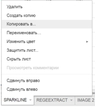
As we have already noted, IMPORTRANGE loads only data, but not the formatting of the source table. How to deal with this? Prepare the soil in advance by copying the formatting from the source sheet. To do this, go to the source sheet and copy it into your book:
After clicking the Copy to ... button, select the book into which you will import data. Usually the table you need is on the Recent tab (if you’ve really recently worked with it).
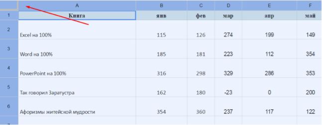
After copying the sheet, select all the data (by clicking on the upper left corner):
And click Delete . All data will disappear, but the formatting will remain. Now you can enter the IMPORTRANGE function and get a full match of the source sheet - both in the data part and in the format part:
IMPORTRANGE as an argument to another function.
IMPORTRANGE can be an argument to another function if the range you are importing is suitable for this role.
Consider a simple example - the average value of sales from a range that is in another document.
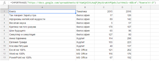
This is the original document. Let the data be added and we need the 2016 average of sales (that is, from cell D2 and all the way down).
First we import this range:
IMPORTRANGE (" docs.google.com/spreadsheets/d/16aKQAIGtLKwQFjWyUGraKAVPQe6cJucYAHoIc-AEEc4 "; "Books! D2: D")
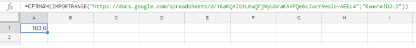
And then use this as an argument of the AVERAGE function:
= AVERAGE (IMPORTRANGE (" docs.google.com/spreadsheets/d/16aKQAIGtLKwQFjWyUGraKAVPQe6cJucYAHoIc-AEEc4 "; "Books! D2: D"))
= AVERAGE (IMPORTRANGE (" docs.google.com/spreadsheets/d/16aKQAIGtLKwQFjWyUGraKAVPQe6cJucYAHoIc-AEEc4 "; "Books! D2: D"))
We get the result, which will be updated when adding new lines in the source file in column D.
IMAGE: add images to cells
The IMAGE feature allows you to add images to your Google Spreadsheets cells.
The function has the following syntax:
IMAGE (URL, [mode], [height], [width])
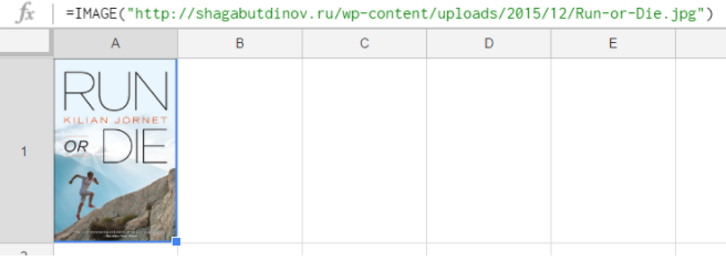
URL is the only required argument. This is a link to the image. The link can be specified directly in the formula, taking in quotes:
= IMAGE (“http://shagabutdinov.ru/wp-content/uploads/2015/12/Run-or-Die.jpg”)
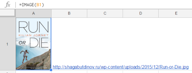
Or put a link to the cell in which the link is stored:
= IMAGE (B1)
The latter option is more convenient in most cases. So, if you have a list of books and links to covers, one formula is enough to display them all:
In practice, it happens that links to images are stored on a separate sheet, and you get them using the VLOOKUP function or something else.
The mode argument can take four values (if you omit it, the first will be the default):
- the image is stretched to the size of the cell while maintaining the aspect ratio;
- the image is stretched without preserving the aspect ratio, completely filling
- The image is inserted with the original size;
- You specify the image size in the third and fourth arguments of the function [height] and [width]. [height], [width], respectively, are needed only if the value of the argument is mode = 4. They are specified in pixels.
Let's see how images look in practice with four different values of the mode argument:
The fourth mode can be convenient if you need to select the exact image size in pixels by changing the height and width parameters. The picture will be immediately updated.
Note that for all modes except the second, there may be empty areas in the cell, and they can be filled with color:
GOOGLETRANSLATE and DETECTLANGUAGE: translate the text in cells
In Google Spreadsheets, there is an interesting function GOOGLETRANSLATE, which allows you to translate text directly into cells:
The syntax of the function is as follows:
GOOGLETRANSLATE (text, [source_language], [target_language])
text is the text to be translated. You can take the text in quotes and write directly into the formula, but it is more convenient to refer to the cell in which the text is written.
[source_language] - the language from which we translate;
[target_language] is the language we translate into.
The second and third arguments are given by a two-digit code: es, fr, en, ru. They can also be specified in the function itself, but can be taken from the cell, and the source text language can be automatically determined.
And what if we want to translate into different languages? And at the same time we do not want to specify the source language manually every time?
This is where the DETECTLANGUAGE function comes in handy. It has a single argument — the text whose language is to be determined:
As with any other function, the beauty here is in automation. You can quickly change the text or language; quickly translate one phrase into 10 languages and so on. Of course, we understand that this is the text of the online translator - the quality will be appropriate.
Yevgeny Namokonov and Renat Shagabutdinov, and we also lead a channel in a telegram, where we analyze different cases with Google Spreadsheets, if you are interested, look in on a visit, you can find the link in my profile.
Source: https://habr.com/ru/post/331360/
All Articles