The implementation of the algorithm A *

This article is a continuation of my introduction to the A * algorithm . In it, I showed how wide the search is implemented, Dijkstra's algorithm, the greedy search for the best first match, and A *. I tried to simplify the explanation as much as possible.
Graph search is a family of similar algorithms. There are many variations of algorithms and their implementations. Treat the code of this article as a starting point, and not the final version of the algorithm, suitable for all situations.
1. Implementation in Python
Below I will explain most of the code. The implementation.py file is somewhat wider. The code uses Python 3 , so if you are using Python 2, you will need to change the
super() call and the print function with analogues from Python 2.')
1.1 Search in width
Let's implement a wide Python search. The first article shows the Python code for the search algorithm, but we also need to determine the graph with which we will work. Here are the abstractions I use:
Count : a data structure that can report the neighbors of each point (see this tutorial )
Points (locations) : a simple value (int, string, tuple, etc.) marking the points in the graph
Search : an algorithm that receives a graph, a starting point and (optionally) an endpoint that calculates useful information (visited, a pointer to the parent element, a distance) for some or all of the points
Queue : data structure used by the search algorithm to select the order in which the points are processed.
In the first article, I mainly looked at the search . In this article I will explain everything else necessary to create a fully working program. Let's start with the graph :
class SimpleGraph: def __init__(self): self.edges = {} def neighbors(self, id): return self.edges[id] Yes, and that's all we need! You may ask: where is the Node object? Answer: I rarely use the node object. It seems to me more simple to use integers, strings or tuples as points, and then use arrays or hash tables to take points as indices.
Notice that the edges have a direction : we may have an edge from A to B, but there may not be an edge from B to A. In game cards, the edges are mostly bi-directional, but sometimes there are one-way doors or jumping from ledges, which are designated as directional edges. Let's create an example of a graph where the points will be denoted by the letters AE.

For each point you need a list of points to which it leads:
example_graph = SimpleGraph() example_graph.edges = { 'A': ['B'], 'B': ['A', 'C', 'D'], 'C': ['A'], 'D': ['E', 'A'], 'E': ['B'] } Before using the search algorithm, we need to set the queue :
import collections class Queue: def __init__(self): self.elements = collections.deque() def empty(self): return len(self.elements) == 0 def put(self, x): self.elements.append(x) def get(self): return self.elements.popleft() This queue class is simply a wrapper around the built-in
collections.deque class. In your code, you can use deque directly.Let's try using our example graph with this queue and a wide search code from the previous article:
from implementation import * def breadth_first_search_1(graph, start): # , frontier = Queue() frontier.put(start) visited = {} visited[start] = True while not frontier.empty(): current = frontier.get() print("Visiting %r" % current) for next in graph.neighbors(current): if next not in visited: frontier.put(next) visited[next] = True breadth_first_search_1(example_graph, 'A') Visiting 'A'
Visiting 'B'
Visiting 'C'
Visiting 'D'
Visiting 'E'Grids can also be expressed as graphs. Now I define a new graph
SquareGrid , with a tuple (int, int) points . Instead of storing the edges explicitly, we will compute them as neighbors . class SquareGrid: def __init__(self, width, height): self.width = width self.height = height self.walls = [] def in_bounds(self, id): (x, y) = id return 0 <= x < self.width and 0 <= y < self.height def passable(self, id): return id not in self.walls def neighbors(self, id): (x, y) = id results = [(x+1, y), (x, y-1), (x-1, y), (x, y+1)] if (x + y) % 2 == 0: results.reverse() # results = filter(self.in_bounds, results) results = filter(self.passable, results) return results Let's check it on the first grid from the previous article:
from implementation import * g = SquareGrid(30, 15) g.walls = DIAGRAM1_WALLS # long, [(21, 0), (21, 2), ...] draw_grid(g) . . . . . . . . . . . . . . . . . . . . . ####. . . . . . .
. . . . . . . . . . . . . . . . . . . . . ####. . . . . . .
. . . . . . . . . . . . . . . . . . . . . ####. . . . . . .
. . . ####. . . . . . . . . . . . . . . . ####. . . . . . .
. . . ####. . . . . . . . ####. . . . . . ####. . . . . . .
. . . ####. . . . . . . . ####. . . . . . ##########. . . .
. . . ####. . . . . . . . ####. . . . . . ##########. . . .
. . . ####. . . . . . . . ####. . . . . . . . . . . . . . .
. . . ####. . . . . . . . ####. . . . . . . . . . . . . . .
. . . ####. . . . . . . . ####. . . . . . . . . . . . . . .
. . . ####. . . . . . . . ####. . . . . . . . . . . . . . .
. . . ####. . . . . . . . ####. . . . . . . . . . . . . . .
. . . . . . . . . . . . . ####. . . . . . . . . . . . . . .
. . . . . . . . . . . . . ####. . . . . . . . . . . . . . .
. . . . . . . . . . . . . ####. . . . . . . . . . . . . . .To recreate the paths, we need to save the point from which we came, so I renamed
visited (True / False) to came_from (point): from implementation import * def breadth_first_search_2(graph, start): # "came_from" frontier = Queue() frontier.put(start) came_from = {} came_from[start] = None while not frontier.empty(): current = frontier.get() for next in graph.neighbors(current): if next not in came_from: frontier.put(next) came_from[next] = current return came_from g = SquareGrid(30, 15) g.walls = DIAGRAM1_WALLS parents = breadth_first_search_2(g, (8, 7)) draw_grid(g, width=2, point_to=parents, start=(8, 7)) → → → → ↓ ↓ ↓ ↓ ↓ ↓ ↓ ↓ ↓ ↓ ↓ ↓ ← ← ← ← ← ####↓ ↓ ↓ ↓ ↓ ↓ ↓
→ → → → → ↓ ↓ ↓ ↓ ↓ ↓ ↓ ↓ ↓ ↓ ← ← ← ← ← ← ####↓ ↓ ↓ ↓ ↓ ↓ ↓
→ → → → → ↓ ↓ ↓ ↓ ↓ ↓ ↓ ↓ ↓ ← ← ← ← ← ← ← ####→ ↓ ↓ ↓ ↓ ↓ ↓
→ → ↑ ####↓ ↓ ↓ ↓ ↓ ↓ ↓ ↓ ← ← ← ← ← ← ← ← ####→ → ↓ ↓ ↓ ↓ ↓
→ ↑ ↑ ####→ ↓ ↓ ↓ ↓ ↓ ↓ ← ####↑ ← ← ← ← ← ####→ → → ↓ ↓ ↓ ↓
↑ ↑ ↑ ####→ → ↓ ↓ ↓ ↓ ← ← ####↑ ↑ ← ← ← ← ##########↓ ↓ ↓ ←
↑ ↑ ↑ ####→ → → ↓ ↓ ← ← ← ####↑ ↑ ↑ ← ← ← ##########↓ ↓ ← ←
↑ ↑ ↑ ####→ → → A ← ← ← ← ####↑ ↑ ↑ ↑ ← ← ← ← ← ← ← ← ← ← ←
↓ ↓ ↓ ####→ → ↑ ↑ ↑ ← ← ← ####↑ ↑ ↑ ↑ ↑ ← ← ← ← ← ← ← ← ← ←
↓ ↓ ↓ ####→ ↑ ↑ ↑ ↑ ↑ ← ← ####↑ ↑ ↑ ↑ ↑ ↑ ← ← ← ← ← ← ← ← ←
↓ ↓ ↓ ####↑ ↑ ↑ ↑ ↑ ↑ ↑ ← ####↑ ↑ ↑ ↑ ↑ ↑ ↑ ← ← ← ← ← ← ← ←
→ ↓ ↓ ####↑ ↑ ↑ ↑ ↑ ↑ ↑ ↑ ####↑ ↑ ↑ ↑ ↑ ↑ ↑ ↑ ← ← ← ← ← ← ←
→ → → → → ↑ ↑ ↑ ↑ ↑ ↑ ↑ ↑ ####↑ ↑ ↑ ↑ ↑ ↑ ↑ ↑ ↑ ← ← ← ← ← ←
→ → → → ↑ ↑ ↑ ↑ ↑ ↑ ↑ ↑ ↑ ####↑ ↑ ↑ ↑ ↑ ↑ ↑ ↑ ↑ ↑ ← ← ← ← ←
→ → → ↑ ↑ ↑ ↑ ↑ ↑ ↑ ↑ ↑ ↑ ####↑ ↑ ↑ ↑ ↑ ↑ ↑ ↑ ↑ ↑ ↑ ← ← ← ←In some implementations, by creating a Node object, internal storage is used to store
came_from and other values for each node of the graph. Instead, I decided to use external storage by creating a single table of hashes for storing came_from all nodes of the graph. If you know that the points of your map have integer indices, then there is another option - use the array for storing the came_from .1.2 Early exit
Repeating the code of the previous article, we just need to add the if construct to the main loop. This check is optional for a wide search and Dijkstra algorithm, but is required for a greedy search for the best first match and A *:
from implementation import * def breadth_first_search_3(graph, start, goal): frontier = Queue() frontier.put(start) came_from = {} came_from[start] = None while not frontier.empty(): current = frontier.get() if current == goal: break for next in graph.neighbors(current): if next not in came_from: frontier.put(next) came_from[next] = current return came_from g = SquareGrid(30, 15) g.walls = DIAGRAM1_WALLS parents = breadth_first_search_3(g, (8, 7), (17, 2)) draw_grid(g, width=2, point_to=parents, start=(8, 7), goal=(17, 2)) . → → → ↓ ↓ ↓ ↓ ↓ ↓ ↓ ↓ ↓ ↓ ↓ ↓ ← . . . . ####. . . . . . .
→ → → → → ↓ ↓ ↓ ↓ ↓ ↓ ↓ ↓ ↓ ↓ ← ← ← . . . ####. . . . . . .
→ → → → → ↓ ↓ ↓ ↓ ↓ ↓ ↓ ↓ ↓ ← ← ← Z . . . ####. . . . . . .
→ → ↑ ####↓ ↓ ↓ ↓ ↓ ↓ ↓ ↓ ← ← ← ← ← ← . . ####. . . . . . .
. ↑ ↑ ####→ ↓ ↓ ↓ ↓ ↓ ↓ ← ####↑ ← ← . . . ####. . . . . . .
. . ↑ ####→ → ↓ ↓ ↓ ↓ ← ← ####↑ ↑ . . . . ##########. . . .
. . . ####→ → → ↓ ↓ ← ← ← ####↑ . . . . . ##########. . . .
. . . ####→ → → A ← ← ← ← ####. . . . . . . . . . . . . . .
. . . ####→ → ↑ ↑ ↑ ← ← ← ####. . . . . . . . . . . . . . .
. . ↓ ####→ ↑ ↑ ↑ ↑ ↑ ← ← ####. . . . . . . . . . . . . . .
. ↓ ↓ ####↑ ↑ ↑ ↑ ↑ ↑ ↑ ← ####. . . . . . . . . . . . . . .
→ ↓ ↓ ####↑ ↑ ↑ ↑ ↑ ↑ ↑ ↑ ####. . . . . . . . . . . . . . .
→ → → → → ↑ ↑ ↑ ↑ ↑ ↑ ↑ ↑ ####. . . . . . . . . . . . . . .
→ → → → ↑ ↑ ↑ ↑ ↑ ↑ ↑ ↑ ↑ ####. . . . . . . . . . . . . . .
. → → ↑ ↑ ↑ ↑ ↑ ↑ ↑ ↑ ↑ ↑ ####. . . . . . . . . . . . . . .As we can see, the algorithm stops when it finds a target
Z1.3 Dijkstra's Algorithm
This adds complexity to the algorithm, because we will start processing the points in an improved order, and not just “first entered, first out.” What principle will we use?
- Count need to know the cost of movement.
- Queues need to return nodes in a different order.
- The search should track this value in the graph and transfer it to the queue.
1.3.1 Weights Graph
I'm going to add the
cost(from_node, to_node) function cost(from_node, to_node) , which tells us the cost of moving from from_node to its neighbor to_node . In this forest map, I decided that movement would depend only on to_node , but there are other types of movement using both nodes . An alternative to the implementation will be to merge it into the function neighbors . class GridWithWeights(SquareGrid): def __init__(self, width, height): super().__init__(width, height) self.weights = {} def cost(self, from_node, to_node): return self.weights.get(to_node, 1) 1.3.2 Priority Queue
The priority queue associates with each element a number called a “priority”. When returning an item, it selects the item with the lowest number.
insert : adds an item to the queue
remove : removes the element with the smallest number
reprioritize : (optional) changes the priority of an existing item to a lower number.
Here is a fairly fast priority queue that uses a binary heap , but does not support reprioritize. To get the correct order, we use a tuple (priority, element). When you insert an item that is already in the queue, we get a duplicate. I will explain why this suits us in the “Optimization” section.
import heapq class PriorityQueue: def __init__(self): self.elements = [] def empty(self): return len(self.elements) == 0 def put(self, item, priority): heapq.heappush(self.elements, (priority, item)) def get(self): return heapq.heappop(self.elements)[1] 1.3.3 Search
There is a tricky moment of implementation: since we add the cost of movement, there is the likelihood of re-visiting a point with a better
cost_so_far . This means that the line if next not in came_from will not work. Instead, we need to check whether the cost has decreased since the last visit. (In the original version of the article, I did not check it, but my code still worked. I wrote notes about this error .)This map with the forest is taken from the previous article .
def dijkstra_search(graph, start, goal): frontier = PriorityQueue() frontier.put(start, 0) came_from = {} cost_so_far = {} came_from[start] = None cost_so_far[start] = 0 while not frontier.empty(): current = frontier.get() if current == goal: break for next in graph.neighbors(current): new_cost = cost_so_far[current] + graph.cost(current, next) if next not in cost_so_far or new_cost < cost_so_far[next]: cost_so_far[next] = new_cost priority = new_cost frontier.put(next, priority) came_from[next] = current return came_from, cost_so_far After the search you need to build a path:
def reconstruct_path(came_from, start, goal): current = goal path = [current] while current != start: current = came_from[current] path.append(current) path.append(start) # path.reverse() # return path Although the ways are better perceived as a sequence of edges, it is more convenient to store as a sequence of nodes. To create the path, let's start from the end and follow the
came_from map pointing to the previous node. When we reach the beginning, it's done. This is the return path, so at the end of reconstruct_path we call reverse() if we need to store it in a direct sequence. In fact, it is sometimes more convenient to store the path in reverse. In addition, it is sometimes convenient to keep the starting node in the list.Let's try:
from implementation import * came_from, cost_so_far = dijkstra_search(diagram4, (1, 4), (7, 8)) draw_grid(diagram4, width=3, point_to=came_from, start=(1, 4), goal=(7, 8)) print() draw_grid(diagram4, width=3, number=cost_so_far, start=(1, 4), goal=(7, 8)) print() draw_grid(diagram4, width=3, path=reconstruct_path(came_from, start=(1, 4), goal=(7, 8))) ↓ ↓ ← ← ← ← ← ← ← ←
↓ ↓ ← ← ← ↑ ↑ ← ← ←
↓ ↓ ← ← ← ← ↑ ↑ ← ←
↓ ↓ ← ← ← ← ← ↑ ↑ .
→ A ← ← ← ← . . . .
↑ ↑ ← ← ← ← . . . .
↑ ↑ ← ← ← ← ← . . .
↑ #########↑ ← ↓ . . .
↑ #########↓ ↓ ↓ Z . .
↑ ← ← ← ← ← ← ← ← .
5 4 5 6 7 8 9 10 11 12
4 3 4 5 10 13 10 11 12 13
3 2 3 4 9 14 15 12 13 14
2 1 2 3 8 13 18 17 14 .
1 A 1 6 11 16 . . . .
2 1 2 7 12 17 . . . .
3 2 3 4 9 14 19 . . .
4 #########14 19 18 . . .
5 #########15 16 13 Z . .
6 7 8 9 10 11 12 13 14 .
. . . . . . . . . .
. . . . . . . . . .
. . . . . . . . . .
. . . . . . . . . .
@ @ . . . . . . . .
@ . . . . . . . . .
@ . . . . . . . . .
@ #########. . . . . .
@ #########. . @ @ . .
@ @ @ @ @ @ @ . . .The
if next not in cost_so_far or new_cost < cost_so_far[next] can be simplified to if new_cost < cost_so_far.get(next, Infinity) , but I didn’t want to explain get() Python in the last article, so I left it as it is. You can also use collections.defaultdict with a default infinity value.1.4 Search A *
And the greedy search for the best first match, and A * use a heuristic function. The only difference is that A * uses both heuristics and ordering from the Dijkstra algorithm. Here I will show A *.
def heuristic(a, b): (x1, y1) = a (x2, y2) = b return abs(x1 - x2) + abs(y1 - y2) def a_star_search(graph, start, goal): frontier = PriorityQueue() frontier.put(start, 0) came_from = {} cost_so_far = {} came_from[start] = None cost_so_far[start] = 0 while not frontier.empty(): current = frontier.get() if current == goal: break for next in graph.neighbors(current): new_cost = cost_so_far[current] + graph.cost(current, next) if next not in cost_so_far or new_cost < cost_so_far[next]: cost_so_far[next] = new_cost priority = new_cost + heuristic(goal, next) frontier.put(next, priority) came_from[next] = current return came_from, cost_so_far Let's try:
from implementation import * came_from, cost_so_far = a_star_search(diagram4, (1, 4), (7, 8)) draw_grid(diagram4, width=3, point_to=came_from, start=(1, 4), goal=(7, 8)) print() draw_grid(diagram4, width=3, number=cost_so_far, start=(1, 4), goal=(7, 8)) . . . . . . . . . .
. ↓ ↓ ↓ . . . . . .
↓ ↓ ↓ ↓ ← . . . . .
↓ ↓ ↓ ← ← . . . . .
→ A ← ← ← . . . . .
→ ↑ ← ← ← . . . . .
→ ↑ ← ← ← ← . . . .
↑ #########↑ . ↓ . . .
↑ #########↓ ↓ ↓ Z . .
↑ ← ← ← ← ← ← ← . .
. . . . . . . . . .
. 3 4 5 . . . . . .
3 2 3 4 9 . . . . .
2 1 2 3 8 . . . . .
1 A 1 6 11 . . . . .
2 1 2 7 12 . . . . .
3 2 3 4 9 14 . . . .
4 #########14 . 18 . . .
5 #########15 16 13 Z . .
6 7 8 9 10 11 12 13 . .1.4.1 Straightened paths
If you implement this code in your own project, you may find that some of the paths are not as “straight” as we would like. This is normal . When using grids , and especially grids, in which each step has the same cost of movement, you will get equal options : many ways have exactly the same value. A * selects one of many shortcuts, and very often it does not look very nice . You can use a fast hack, eliminating equivalent options , but it is not always fully suitable. It would be better to change the map view , which will make A * much faster and create more direct and pleasant paths. However, this is suitable for static maps in which each step has one movement cost. For the demo on my page I use a fast hack, but it only works with my slow priority queue. If you switch to a faster priority queue, you will need another quick hack.
2 Implementation in C ++
Note: to perform part of the example code, add redblobgames / pathfinding / a-star / implementation.cpp . I use C ++ 11 for this code, so if you are using an older version of the C ++ standard, you will have to partially change it.
2.1 Search in width
First read the section on Python. In this section there will be a code, but there will not be the same explanations. First we add the general class of the graph:
template<typename L> struct SimpleGraph { typedef L Location; typedef typename vector<Location>::iterator iterator; unordered_map<Location, vector<Location> > edges; inline const vector<Location> neighbors(Location id) { return edges[id]; } }; and the same example of a graph from Python code that uses
char to mark points: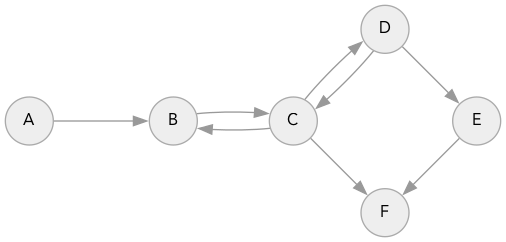
SimpleGraph<char> example_graph {{ {'A', {'B'}}, {'B', {'A', 'C', 'D'}}, {'C', {'A'}}, {'D', {'E', 'A'}}, {'E', {'B'}} }}; Instead of defining the queue class, we use the class from the standard C ++ library. Now we can try a wider search:
#include "redblobgames/pathfinding/a-star/implementation.cpp" template<typename Graph> void breadth_first_search(Graph graph, typename Graph::Location start) { typedef typename Graph::Location Location; queue<Location> frontier; frontier.push(start); unordered_set<Location> visited; visited.insert(start); while (!frontier.empty()) { auto current = frontier.front(); frontier.pop(); std::cout << "Visiting " << current << std::endl; for (auto& next : graph.neighbors(current)) { if (!visited.count(next)) { frontier.push(next); visited.insert(next); } } } } int main() { breadth_first_search(example_graph, 'A'); } Visiting A
Visiting B
Visiting C
Visiting D
Visiting EThe code is slightly longer than in Python, but this is quite normal.
What about squares grids? I will define another class of the graph. Notice that it is not related to the previous class of the graph. I use patterns, not inheritance. The graph should only provide a typedef
Location and a neighbors function. struct SquareGrid { typedef tuple<int,int> Location; static array<Location, 4> DIRS; int width, height; unordered_set<Location> walls; SquareGrid(int width_, int height_) : width(width_), height(height_) {} inline bool in_bounds(Location id) const { int x, y; tie (x, y) = id; return 0 <= x && x < width && 0 <= y && y < height; } inline bool passable(Location id) const { return !walls.count(id); } vector<Location> neighbors(Location id) const { int x, y, dx, dy; tie (x, y) = id; vector<Location> results; for (auto dir : DIRS) { tie (dx, dy) = dir; Location next(x + dx, y + dy); if (in_bounds(next) && passable(next)) { results.push_back(next); } } if ((x + y) % 2 == 0) { // std::reverse(results.begin(), results.end()); } return results; } }; array<SquareGrid::Location, 4> SquareGrid::DIRS {Location{1, 0}, Location{0, -1}, Location{-1, 0}, Location{0, 1}}; In the auxiliary
implementation.cpp file, I defined a function for grid drawing: #include "redblobgames/pathfinding/a-star/implementation.cpp" int main() { SquareGrid grid = make_diagram1(); draw_grid(grid, 2); } . . . . . . . . . . . . . . . . . . . . . ####. . . . . . .
. . . . . . . . . . . . . . . . . . . . . ####. . . . . . .
. . . . . . . . . . . . . . . . . . . . . ####. . . . . . .
. . . ####. . . . . . . . . . . . . . . . ####. . . . . . .
. . . ####. . . . . . . . ####. . . . . . ####. . . . . . .
. . . ####. . . . . . . . ####. . . . . . ##########. . . .
. . . ####. . . . . . . . ####. . . . . . ##########. . . .
. . . ####. . . . . . . . ####. . . . . . . . . . . . . . .
. . . ####. . . . . . . . ####. . . . . . . . . . . . . . .
. . . ####. . . . . . . . ####. . . . . . . . . . . . . . .
. . . ####. . . . . . . . ####. . . . . . . . . . . . . . .
. . . ####. . . . . . . . ####. . . . . . . . . . . . . . .
. . . . . . . . . . . . . ####. . . . . . . . . . . . . . .
. . . . . . . . . . . . . ####. . . . . . . . . . . . . . .
. . . . . . . . . . . . . ####. . . . . . . . . . . . . . .Let's do a wider search again by tracking
came_from : #include "redblobgames/pathfinding/a-star/implementation.cpp" template<typename Graph> unordered_map<typename Graph::Location, typename Graph::Location> breadth_first_search(Graph graph, typename Graph::Location start) { typedef typename Graph::Location Location; queue<Location> frontier; frontier.push(start); unordered_map<Location, Location> came_from; came_from[start] = start; while (!frontier.empty()) { auto current = frontier.front(); frontier.pop(); for (auto& next : graph.neighbors(current)) { if (!came_from.count(next)) { frontier.push(next); came_from[next] = current; } } } return came_from; } int main() { SquareGrid grid = make_diagram1(); auto parents = breadth_first_search(grid, std::make_tuple(7, 8)); draw_grid(grid, 2, nullptr, &parents); } → → → → ↓ ↓ ↓ ↓ ↓ ↓ ↓ ↓ ↓ ↓ ↓ ↓ ← ← ← ← ← ####↓ ↓ ↓ ↓ ↓ ↓ ↓
→ → → → → ↓ ↓ ↓ ↓ ↓ ↓ ↓ ↓ ↓ ↓ ← ← ← ← ← ← ####↓ ↓ ↓ ↓ ↓ ↓ ↓
→ → → → → ↓ ↓ ↓ ↓ ↓ ↓ ↓ ↓ ↓ ← ← ← ← ← ← ← ####→ ↓ ↓ ↓ ↓ ↓ ↓
→ → ↑ ####↓ ↓ ↓ ↓ ↓ ↓ ↓ ↓ ← ← ← ← ← ← ← ← ####→ → ↓ ↓ ↓ ↓ ↓
→ ↑ ↑ ####↓ ↓ ↓ ↓ ↓ ↓ ↓ ← ####↑ ← ← ← ← ← ####→ → → ↓ ↓ ↓ ↓
↑ ↑ ↑ ####↓ ↓ ↓ ↓ ↓ ↓ ← ← ####↑ ↑ ← ← ← ← ##########↓ ↓ ↓ ←
↑ ↑ ↑ ####→ ↓ ↓ ↓ ↓ ← ← ← ####↑ ↑ ↑ ← ← ← ##########↓ ↓ ← ←
↓ ↓ ↓ ####→ → ↓ ↓ ← ← ← ← ####↑ ↑ ↑ ↑ ← ← ← ← ← ← ← ← ← ← ←
↓ ↓ ↓ ####→ → * ← ← ← ← ← ####↑ ↑ ↑ ↑ ↑ ← ← ← ← ← ← ← ← ← ←
↓ ↓ ↓ ####→ ↑ ↑ ↑ ← ← ← ← ####↑ ↑ ↑ ↑ ↑ ↑ ← ← ← ← ← ← ← ← ←
↓ ↓ ↓ ####↑ ↑ ↑ ↑ ↑ ← ← ← ####↑ ↑ ↑ ↑ ↑ ↑ ↑ ← ← ← ← ← ← ← ←
→ ↓ ↓ ####↑ ↑ ↑ ↑ ↑ ↑ ← ← ####↑ ↑ ↑ ↑ ↑ ↑ ↑ ↑ ← ← ← ← ← ← ←
→ → → → → ↑ ↑ ↑ ↑ ↑ ↑ ↑ ← ####↑ ↑ ↑ ↑ ↑ ↑ ↑ ↑ ↑ ← ← ← ← ← ←
→ → → → ↑ ↑ ↑ ↑ ↑ ↑ ↑ ↑ ↑ ####↑ ↑ ↑ ↑ ↑ ↑ ↑ ↑ ↑ ↑ ← ← ← ← ←
→ → → ↑ ↑ ↑ ↑ ↑ ↑ ↑ ↑ ↑ ↑ ####↑ ↑ ↑ ↑ ↑ ↑ ↑ ↑ ↑ ↑ ↑ ← ← ← ←In some implementations, internal storage is used and a Node object is created to store
came_from and other values for each node of the graph. I chose to use external storage , creating a single std::unordered_map for storing came_from for all nodes of the graph. If you know that the points of your map have integer indices, then there is another option - use a one-dimensional or two-dimensional array / vector to store came_from and other values.2.1.1 TODO: struct points
In this code, I use
std::tuple C ++, because I used tuples in my Python code. However, the tuples are unfamiliar to most C ++ programmers. It will be a little longer to define a struct with {x, y}, because you need to define a constructor, a copy constructor, an assignment operator, and an equality comparison along with a hash function, but such code will be more familiar to most C ++ programmers. You will need to change it.Another option (I use it in my code) is to encode {x, y} as an
int . T If the A * code always has a dense set of integer-valued values instead of arbitrary Location types, this allows for additional optimizations. You can use arrays for different sets, not hashes tables. You can leave most of them uninitialized. For those arrays that need to be initialized anew each time, you can make them permanent for A * calls (possibly using local stream storage) and reinitialize only those parts of the array that were used in the previous call. This is a more complicated technique that I do not want to use in the tutorial of the initial level.2.2 Early exit
As in the Python version, we just need to add a parameter to the function and check the main loop:
#include "redblobgames/pathfinding/a-star/implementation.cpp" template<typename Graph> unordered_map<typename Graph::Location, typename Graph::Location> breadth_first_search(const Graph& graph, typename Graph::Location start, typename Graph::Location goal) { typedef typename Graph::Location Location; queue<Location> frontier; frontier.push(start); unordered_map<Location, Location> came_from; came_from[start] = start; while (!frontier.empty()) { auto current = frontier.front(); frontier.pop(); if (current == goal) { break; } for (auto& next : graph.neighbors(current)) { if (!came_from.count(next)) { frontier.push(next); came_from[next] = current; } } } return came_from; } int main() { SquareGrid grid = make_diagram1(); auto parents = breadth_first_search(grid, SquareGrid::Location{8, 7}, SquareGrid::Location{17, 2}); draw_grid(grid, 2, nullptr, &parents); } . → → → ↓ ↓ ↓ ↓ ↓ ↓ ↓ ↓ ↓ ↓ ↓ ↓ ← . . . . ####. . . . . . .
→ → → → → ↓ ↓ ↓ ↓ ↓ ↓ ↓ ↓ ↓ ↓ ← ← ← . . . ####. . . . . . .
→ → → → → ↓ ↓ ↓ ↓ ↓ ↓ ↓ ↓ ↓ ← ← ← ← . . . ####. . . . . . .
→ → ↑ ####↓ ↓ ↓ ↓ ↓ ↓ ↓ ↓ ← ← ← ← ← ← . . ####. . . . . . .
. ↑ ↑ ####→ ↓ ↓ ↓ ↓ ↓ ↓ ← ####↑ ← ← . . . ####. . . . . . .
. . ↑ ####→ → ↓ ↓ ↓ ↓ ← ← ####↑ ↑ . . . . ##########. . . .
. . . ####→ → → ↓ ↓ ← ← ← ####↑ . . . . . ##########. . . .
. . . ####→ → → * ← ← ← ← ####. . . . . . . . . . . . . . .
. . . ####→ → ↑ ↑ ↑ ← ← ← ####. . . . . . . . . . . . . . .
. . ↓ ####→ ↑ ↑ ↑ ↑ ↑ ← ← ####. . . . . . . . . . . . . . .
. ↓ ↓ ####↑ ↑ ↑ ↑ ↑ ↑ ↑ ← ####. . . . . . . . . . . . . . .
→ ↓ ↓ ####↑ ↑ ↑ ↑ ↑ ↑ ↑ ↑ ####. . . . . . . . . . . . . . .
→ → → → → ↑ ↑ ↑ ↑ ↑ ↑ ↑ ↑ ####. . . . . . . . . . . . . . .
→ → → → ↑ ↑ ↑ ↑ ↑ ↑ ↑ ↑ ↑ ####. . . . . . . . . . . . . . .
. → → ↑ ↑ ↑ ↑ ↑ ↑ ↑ ↑ ↑ ↑ ####. . . . . . . . . . . . . . .2.3 Dijkstra’s Algorithm
2.3.1 Weights Count
We have a grid with a list of forest tiles, the cost of movement on which is 5. In this forest map, I decided to perform movement only depending on
to_node , but there are other types of movement using both nodes . struct GridWithWeights: SquareGrid { unordered_set<Location> forests; GridWithWeights(int w, int h): SquareGrid(w, h) {} double cost(Location from_node, Location to_node) const { return forests.count(to_node) ? 5 : 1; } }; 2.3.2 Priority Queue
We need a priority queue. In C ++, there is a
priority_queue class that uses a binary heap, but without a priority change operation. I use a pair (priority, element) for the elements of the queue to get the correct order. By default, the C ++ priority queue first returns the maximum element using the std::less comparator. We need a minimal element, so I use the std::greater comparator. template<typename T, typename priority_t> struct PriorityQueue { typedef pair<priority_t, T> PQElement; priority_queue<PQElement, vector<PQElement>, std::greater<PQElement>> elements; inline bool empty() const { return elements.empty(); } inline void put(T item, priority_t priority) { elements.emplace(priority, item); } inline T get() { T best_item = elements.top().second; elements.pop(); return best_item; } }; In this example code, I wrap the C ++
std::priority_queue , but I think it would be wise to use this class without a wrapper.2.3.3 Search
See the map with the forest from the previous article .
template<typename Graph> void dijkstra_search (const Graph& graph, typename Graph::Location start, typename Graph::Location goal, unordered_map<typename Graph::Location, typename Graph::Location>& came_from, unordered_map<typename Graph::Location, double>& cost_so_far) { typedef typename Graph::Location Location; PriorityQueue<Location, double> frontier; frontier.put(start, 0); came_from[start] = start; cost_so_far[start] = 0; while (!frontier.empty()) { auto current = frontier.get(); if (current == goal) { break; } for (auto& next : graph.neighbors(current)) { double new_cost = cost_so_far[current] + graph.cost(current, next); if (!cost_so_far.count(next) || new_cost < cost_so_far[next]) { cost_so_far[next] = new_cost; came_from[next] = current; frontier.put(next, new_cost); } } } } The types of
cost variables must match the types used in the graph. If you use int , you can use int for variable values and priorities in the priority queue. If you use double , then you also need to use double for them. In this code, I used double , but int could also be used, and the code would work just the same. However, if the cost of the graph edges is stored in double or double is used in heuristics, then double should be used here.And finally, after the search you need to build a path:
template<typename Location> vector<Location> reconstruct_path( Location start, Location goal, unordered_map<Location, Location>& came_from ) { vector<Location> path; Location current = goal; path.push_back(current); while (current != start) { current = came_from[current]; path.push_back(current); } path.push_back(start); // std::reverse(path.begin(), path.end()); return path; } Although the paths are better seen as a sequence of edges, it is convenient to store them as a sequence of nodes. To build the path, let's start from the end and follow the
came_from map pointing to the previous node. The process will end when we reach the beginning. This is a return path, so if you want to store it in a direct form, then at the end of reconstruct_path you need to call reverse() . Sometimes it is more convenient to store the path in reverse. Sometimes it is also useful to keep the starting node in the list.Let's try:
#include "redblobgames/pathfinding/a-star/implementation.cpp" int main() { GridWithWeights grid = make_diagram4(); SquareGrid::Location start{1, 4}; SquareGrid::Location goal{8, 5}; unordered_map<SquareGrid::Location, SquareGrid::Location> came_from; unordered_map<SquareGrid::Location, double> cost_so_far; dijkstra_search(grid, start, goal, came_from, cost_so_far); draw_grid(grid, 2, nullptr, &came_from); std::cout << std::endl; draw_grid(grid, 3, &cost_so_far, nullptr); std::cout << std::endl; vector<SquareGrid::Location> path = reconstruct_path(start, goal, came_from); draw_grid(grid, 3, nullptr, nullptr, &path); } ↓ ↓ ← ← ← ← ← ← ← ←
↓ ↓ ← ← ← ↑ ↑ ← ← ←
↓ ↓ ← ← ← ← ↑ ↑ ← ←
↓ ↓ ← ← ← ← ← ↑ ↑ ←
→ * ← ← ← ← ← → ↑ ←
↑ ↑ ← ← ← ← . ↓ ↑ .
↑ ↑ ← ← ← ← ← ↓ ← .
↑ ######↑ ← ↓ ↓ ← .
↑ ######↓ ↓ ↓ ← ← ←
↑ ← ← ← ← ← ← ← ← ←
5 4 5 6 7 8 9 10 11 12
4 3 4 5 10 13 10 11 12 13
3 2 3 4 9 14 15 12 13 14
2 1 2 3 8 13 18 17 14 15
1 0 1 6 11 16 21 20 15 16
2 1 2 7 12 17 . 21 16 .
3 2 3 4 9 14 19 16 17 .
4 #########14 19 18 15 16 .
5 #########15 16 13 14 15 16
6 7 8 9 10 11 12 13 14 15
. @ @ @ @ @ @ . . .
. @ . . . . @ @ . .
. @ . . . . . @ @ .
. @ . . . . . . @ .
. @ . . . . . . @ .
. . . . . . . . @ .
. . . . . . . . . .
. #########. . . . . .
. #########. . . . . .
. . . . . . . . . .The results do not completely coincide with the results of the Python version, because for the priority queue I use the built-in hash tables, and the iteration order over the hash tables will not be constant.
2.4 Search A *
A * almost completely repeats Dijkstra's algorithm, except for the added heuristic search. Note that the algorithm code can be used not only for grids . Knowledge of grids is in the class of the graph (in this case
SquareGrids) and in the function heuristic. If you replace them, you can use the code of the algorithm A * with any other structure of graphs. inline double heuristic(SquareGrid::Location a, SquareGrid::Location b) { int x1, y1, x2, y2; tie (x1, y1) = a; tie (x2, y2) = b; return abs(x1 - x2) + abs(y1 - y2); } template<typename Graph> void a_star_search (const Graph& graph, typename Graph::Location start, typename Graph::Location goal, unordered_map<typename Graph::Location, typename Graph::Location>& came_from, unordered_map<typename Graph::Location, double>& cost_so_far) { typedef typename Graph::Location Location; PriorityQueue<Location, double> frontier; frontier.put(start, 0); came_from[start] = start; cost_so_far[start] = 0; while (!frontier.empty()) { auto current = frontier.get(); if (current == goal) { break; } for (auto& next : graph.neighbors(current)) { double new_cost = cost_so_far[current] + graph.cost(current, next); if (!cost_so_far.count(next) || new_cost < cost_so_far[next]) { cost_so_far[next] = new_cost; double priority = new_cost + heuristic(next, goal); frontier.put(next, priority); came_from[next] = current; } } } } The type of values
priority, including the type used for the priority queue, must be large enough to contain both the value of the graph ( cost_t) and the heuristic value. For example, if the value of the graph is stored in an int, and the heuristics returns a double, then it is necessary that the priority queue can receive a double. In this code example I use doublefor all three values (cost, heuristics and priority), but I could use and int, because my cost and heuristics have integer values.A small note: it would be more correct to write
frontier.put(start, heuristic(start, goal)), rather thanfrontier.put(start, 0), but here it is not important, because the priority of the initial node does not matter. This is the only node in the priority queue and it is selected and deleted before something is written there. #include "redblobgames/pathfinding/a-star/implementation.cpp" int main() { GridWithWeights grid = make_diagram4(); SquareGrid::Location start{1, 4}; SquareGrid::Location goal{8, 5}; unordered_map<SquareGrid::Location, SquareGrid::Location> came_from; unordered_map<SquareGrid::Location, double> cost_so_far; a_star_search(grid, start, goal, came_from, cost_so_far); draw_grid(grid, 2, nullptr, &came_from); std::cout << std::endl; draw_grid(grid, 3, &cost_so_far, nullptr); std::cout << std::endl; vector<SquareGrid::Location> path = reconstruct_path(start, goal, came_from); draw_grid(grid, 3, nullptr, nullptr, &path); } ↓ ↓ ↓ ↓ ← ← ← ← ← ←
↓ ↓ ↓ ↓ ← ↑ ↑ ← ← ←
↓ ↓ ↓ ↓ ← ← ↑ ↑ ← ←
↓ ↓ ↓ ← ← ← . ↑ ↑ ←
→ * ← ← ← ← . → ↑ ←
→ ↑ ← ← ← ← . . ↑ .
↑ ↑ ↑ ← ← ← . . . .
↑ ######↑ . . . . .
↑ ######. . . . . .
↑ . . . . . . . . .
5 4 5 6 7 8 9 10 11 12
4 3 4 5 10 13 10 11 12 13
3 2 3 4 9 14 15 12 13 14
2 1 2 3 8 13 . 17 14 15
1 0 1 6 11 16 . 20 15 16
2 1 2 7 12 17 . . 16 .
3 2 3 4 9 14 . . . .
4 #########14 . . . . .
5 #########. . . . . .
6 . . . . . . . . .
. . . @ @ @ @ . . .
. . . @ . . @ @ . .
. . . @ . . . @ @ .
. . @ @ . . . . @ .
. @ @ . . . . . @ .
. . . . . . . . @ .
. . . . . . . . . .
. #########. . . . . .
. #########. . . . . .
. . . . . . . . . .2.4.1
, «», . . , , , : . A* , . , . , which will speed up A * much and create more direct and beautiful paths. However, this only works with static maps, in which each step has the same cost of movement. For the demo on my page, I used a fast hack, but it only works with my slow priority queue. If you move to a faster priority queue, then you need another quick hack.
2.4.2 TODO: vector neighbors () should be transmitted
Instead of selecting and returning each time a new vector for neighbors, the A * code should allocate one vector and each time pass it to the neighbors function. In my tests, this made the code much faster.
2.4.3 TODO: eliminate template parameterization
The goal of this page is to create easy-to-understand code, and I believe that parameterizing a template is too difficult to read. Instead, I use several typedefs.
2.4.4 TODO: add requirements
There are two types of graphs (weighted and unweighted), and the search code for the graph does not indicate which type is required.
3 Implementation on C #
These are my first C # programs, so they may be uncharacteristic or stylistically incorrect for this language. These examples are not as complete as the examples in the Python and C ++ sections, but I hope they will be useful. Here is an implementation of a simple graph and search in width:
using System; using System.Collections.Generic; public class Graph<Location> { // string, // NameValueCollection public Dictionary<Location, Location[]> edges = new Dictionary<Location, Location[]>(); public Location[] Neighbors(Location id) { return edges[id]; } }; class BreadthFirstSearch { static void Search(Graph<string> graph, string start) { var frontier = new Queue<string>(); frontier.Enqueue(start); var visited = new HashSet<string>(); visited.Add(start); while (frontier.Count > 0) { var current = frontier.Dequeue(); Console.WriteLine("Visiting {0}", current); foreach (var next in graph.Neighbors(current)) { if (!visited.Contains(next)) { frontier.Enqueue(next); visited.Add(next); } } } } static void Main() { Graph<string> g = new Graph<string>(); g.edges = new Dictionary<string, string[]> { { "A", new [] { "B" } }, { "B", new [] { "A", "C", "D" } }, { "C", new [] { "A" } }, { "D", new [] { "E", "A" } }, { "E", new [] { "B" } } }; Search(g, "A"); } } Here is a graph representing a grid with weighted edges (an example of a forest and walls from the previous article):
using System; using System.Collections.Generic; // A* WeightedGraph L, ** // . . public interface WeightedGraph<L> { double Cost(Location a, Location b); IEnumerable<Location> Neighbors(Location id); } public struct Location { // : Equals , // . , // Equals GetHashCode. public readonly int x, y; public Location(int x, int y) { this.x = x; this.y = y; } } public class SquareGrid : WeightedGraph<Location> { // : , // , , // . public static readonly Location[] DIRS = new [] { new Location(1, 0), new Location(0, -1), new Location(-1, 0), new Location(0, 1) }; public int width, height; public HashSet<Location> walls = new HashSet<Location>(); public HashSet<Location> forests = new HashSet<Location>(); public SquareGrid(int width, int height) { this.width = width; this.height = height; } public bool InBounds(Location id) { return 0 <= id.x && id.x < width && 0 <= id.y && id.y < height; } public bool Passable(Location id) { return !walls.Contains(id); } public double Cost(Location a, Location b) { return forests.Contains(b) ? 5 : 1; } public IEnumerable<Location> Neighbors(Location id) { foreach (var dir in DIRS) { Location next = new Location(id.x + dir.x, id.y + dir.y); if (InBounds(next) && Passable(next)) { yield return next; } } } } public class PriorityQueue<T> { // , // . // C#: https://github.com/dotnet/corefx/issues/574 // // , : // * https://github.com/BlueRaja/High-Speed-Priority-Queue-for-C-Sharp // * http://visualstudiomagazine.com/articles/2012/11/01/priority-queues-with-c.aspx // * http://xfleury.imtqy.com/graphsearch.html // * http://stackoverflow.com/questions/102398/priority-queue-in-net private List<Tuple<T, double>> elements = new List<Tuple<T, double>>(); public int Count { get { return elements.Count; } } public void Enqueue(T item, double priority) { elements.Add(Tuple.Create(item, priority)); } public T Dequeue() { int bestIndex = 0; for (int i = 0; i < elements.Count; i++) { if (elements[i].Item2 < elements[bestIndex].Item2) { bestIndex = i; } } T bestItem = elements[bestIndex].Item1; elements.RemoveAt(bestIndex); return bestItem; } } /* : Python * , . C++ * typedef, int, double * . C# , * double. int, , * , , , * . */ public class AStarSearch { public Dictionary<Location, Location> cameFrom = new Dictionary<Location, Location>(); public Dictionary<Location, double> costSoFar = new Dictionary<Location, double>(); // : A* Location // Heuristic static public double Heuristic(Location a, Location b) { return Math.Abs(ax - bx) + Math.Abs(ay - by); } public AStarSearch(WeightedGraph<Location> graph, Location start, Location goal) { var frontier = new PriorityQueue<Location>(); frontier.Enqueue(start, 0); cameFrom[start] = start; costSoFar[start] = 0; while (frontier.Count > 0) { var current = frontier.Dequeue(); if (current.Equals(goal)) { break; } foreach (var next in graph.Neighbors(current)) { double newCost = costSoFar[current] + graph.Cost(current, next); if (!costSoFar.ContainsKey(next) || newCost < costSoFar[next]) { costSoFar[next] = newCost; double priority = newCost + Heuristic(next, goal); frontier.Enqueue(next, priority); cameFrom[next] = current; } } } } } public class Test { static void DrawGrid(SquareGrid grid, AStarSearch astar) { // cameFrom for (var y = 0; y < 10; y++) { for (var x = 0; x < 10; x++) { Location id = new Location(x, y); Location ptr = id; if (!astar.cameFrom.TryGetValue(id, out ptr)) { ptr = id; } if (grid.walls.Contains(id)) { Console.Write("##"); } else if (ptr.x == x+1) { Console.Write("\u2192 "); } else if (ptr.x == x-1) { Console.Write("\u2190 "); } else if (ptr.y == y+1) { Console.Write("\u2193 "); } else if (ptr.y == y-1) { Console.Write("\u2191 "); } else { Console.Write("* "); } } Console.WriteLine(); } } static void Main() { // " 4" var grid = new SquareGrid(10, 10); for (var x = 1; x < 4; x++) { for (var y = 7; y < 9; y++) { grid.walls.Add(new Location(x, y)); } } grid.forests = new HashSet<Location> { new Location(3, 4), new Location(3, 5), new Location(4, 1), new Location(4, 2), new Location(4, 3), new Location(4, 4), new Location(4, 5), new Location(4, 6), new Location(4, 7), new Location(4, 8), new Location(5, 1), new Location(5, 2), new Location(5, 3), new Location(5, 4), new Location(5, 5), new Location(5, 6), new Location(5, 7), new Location(5, 8), new Location(6, 2), new Location(6, 3), new Location(6, 4), new Location(6, 5), new Location(6, 6), new Location(6, 7), new Location(7, 3), new Location(7, 4), new Location(7, 5) }; // A* var astar = new AStarSearch(grid, new Location(1, 4), new Location(8, 5)); DrawGrid(grid, astar); } } 4 Optimization
When creating the code for the article, I focused on simplicity and applicability, and not on performance. First make the code work, then optimize the speed. Many of the optimizations used by me in real projects are specific to the project, so instead of showing the optimal code, I’ll give you some ideas that you can implement in your own project:
4.1 Count
The biggest optimization you can make is reducing the number of nodes. Recommendation number 1: If you are using a map from grids, then try using a non-grid-based path search graph . This is not always possible, but this option is worth considering.
If the graph has a simple structure (for example, a grid), then calculate the neighbors in the function. If it has a more complex structure (without grids, or a grid with a large number of walls, like in a maze), then store your neighbors in a data structure.
You can also save copy operations on the reuse of an array of neighbors. Instead of performing a return every time, select it once in the search code and pass it to the method of the neighbors graph.
4.2 Queue
, , . , . . . , , .
deque. deque , . Python collections.deque ; C++ deque . : , , .
, . , - . Python heapq ; C++ priority_queue .
Python Queue PriorityQueue , . , , . C++ .
Note that in the Dijkstra algorithm, the priority queue with priorities is stored twice, once in the priority queue, the second is in
cost_so_far, so you can write a priority queue that takes priority from any place. I do not know whether it is worth it.The standard implementation of the Dijkstra algorithm uses priority changes in the priority queue. However, what happens if you do not change the priority? As a result, duplicate elements will appear there. But the algorithm still works.He will re-visit some points more than necessary. There will be more elements in the priority queue than necessary, which slows down work, but data structures that support priority changes also slow down work due to the presence of more elements. See the study “Priority Queues and Dijkstra's Algorithm” by Chen, Chowdheri, Ramachandran, Lan-Roch, and Tonga. This study also recommends considering pairing heaps and other data structures.
If you are thinking of using something instead of a binary heap, first measure the size of the border and the frequency of changing priorities. Profile the code and see if the priority queue is a bottleneck.
I feel that a promising direction is . , , A* . .
f , f+e , e — . 1 5. , f f+5 . , . You can use six blocks or do not sort anything at all! A * creates a wider range of priorities, but still this method is worth considering. And there are more interesting approaches to grouping that can handle a wider range of situations.I have another article on priority queuing data structures .
4.3 Search
Heuristics increase the complexity and cost of CPU time. However, the goal here is to study fewer nodes. In some maps (for example, in labyrinths), heuristics may not add much information, and it may be better to use a simpler algorithm without heuristics.
If your graph as points using integer values, then consider the possibility of using
cost_so_far, visited, came_frometc. a simple array, not a hash table. Since it visitedis a boolean array, you can use a bit vector. Initialize the bit vector for all the IDs, but leave cost_so_farand came_fromuninitialized (if the language allows it). Then initialize them only at the first visit., . , . , . ,
visited[] , 1000 , 100 , , 100 , 1000 .A* (overestimated) heuristics. It seems reasonable. However, I did not carefully consider these implementations. I suppose (but I don’t know for sure) that some elements already visited need to be visited again, even if they have already been removed from the border.
In some implementations, a new node is always inserted into an open set , even if it is already there. This avoids the potentially costly step of checking whether a node is already in an open set. But at the same time, the open set becomes larger / slower and, as a result, will have to evaluate more nodes than necessary. If checking an open set turns out to be costly, then you might want to use this approach. However, in the code I presented, I made the check cheap, and I do not use this approach.
In some implementationsIt does not check whether a new node is better than an existing one in an open set. This avoids potentially costly validation. However, this may lead to an error . On some types of cards you will not find the shortest path if you skip this check. In the code I presented, I perform this check (
new_cost < cost_so_far). This check is cheap because I made the search cost_so_farcheap.5 Troubleshooting
5.1 Wrong paths
If you do not get the shortest path, try the following checks:
- Does the priority queue work correctly? Try stopping the search and retrieving all items from the queue. They must go in order.
- ?
priority, ( , ). - , . , , . , , , .
5.2
Most often, when performing A * on grids, they ask me a question: why do the paths not look straight? If you tell A * that all movements along the grid have equal cost, you get a set of shortest paths of the same length, and the algorithm randomly chooses one of them. The path is short , but it does not look good.
- One solution would be to straighten the paths after the algorithm using the string pulling algorithm.
- Another solution is to direct the path in the right direction by regulating heuristics. There are some cheap tricks that do not work in all situations; here you can read more about this .
- — . A* , , . .
- — , . (: , , , ), «» ( (x+y) % 2 == 1). .
6
- . . :
costw or d l lengthcost_so_farg d distanceheuristichpriorityA* f , f = g + hcame_fromπ parent previous prevfrontierOPENvisited— OPEN CLOSED- , ,
currentnextu , v
- :
- ()
- A*
Source: https://habr.com/ru/post/331220/
All Articles