Typical probability distributions: data scientist cheat sheet

The data scientist has hundreds of probability distributions for every taste. Where to begin?

Data science, whatever it was there - thats something else. You can hear from some guru at your gatherings or hackathons: "A data scientist understands statistics better than any programmer." Applied mathematicians are taking revenge for the fact that statistics are no longer as widely heard as in gold 20s . They even have their own unfunny Venn diagram about it . So, suddenly, you, the programmer, find yourself completely out of work in a conversation about confidence intervals , instead of habitually grumbling at analysts who have never heard of the Apache Bikeshed project in order to distribute formatted comments. For such a situation, to be in the jet and again become the soul of the company - you need an express course on statistics. Maybe not deep enough for you to understand everything, but quite enough so that it might seem at first glance.

Probability distributions are the basis of statistics, just as data structures are the basis of computer science. If you want to speak in the language of a data scientist, you need to start by studying them. In principle, it is possible, if lucky, to do simple analyzes using R or scikit-learn without understanding distributions at all, just as you can write a Java program without understanding hash functions. But sooner or later it will end with tears, mistakes, false results or - much worse - oohs and bulging eyes from senior statisticians.

There are hundreds of different distributions, some of which sound like monsters of medieval legends, such as Muth or Lomax . However, in practice, around 15 are used more or less frequently. What are they, and what clever phrases about them do you need to remember?

So what is the probability distribution?

Something happens all the time: cubes are thrown, it is raining, buses are pulling up. After this something happened, you can be sure of some outcome: the cubes fell to 3 and 4, 2.5 cm of rain fell, the bus arrived after 3 minutes. But up to this point we can only talk about how each outcome is possible. Probability distributions describe how we see the probability of each outcome, which is often much more interesting than knowing only one, the most possible, outcome. Distributions come in different forms, but strictly the same size: the sum of all probabilities in the distribution is always 1.
')
For example, throwing a regular coin has two outcomes: it will fall either as an eagle or as a tail (assuming that it does not land on the edge and the gull does not pull it in the air). Before the throw, we believe that with a chance of 1 to 2 or with a probability of 0.5, she will fall with an eagle. Just like tails. This is the probability distribution of two outcomes of a throw, and if you have carefully read this sentence, then you have already understood the Bernoulli distribution .

Despite the exotic names, common distributions are related to each other in rather intuitive and interesting ways that make them easy to remember and reasonably talk about them. Some naturally follow, for example, from the Bernoulli distribution. Time to show a map of these links.



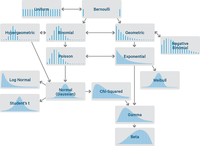
Each distribution is illustrated by an example of its distribution density function (IDF). This article is only about those distributions whose outcomes are single numbers. Therefore, the horizontal axis of each graph is a set of possible outcome numbers. Vertical - the probability of each outcome. Some distributions are discrete — their outcomes must be integers, such as 0 or 5. These are indicated by sparse lines, one for each outcome, with a height corresponding to the probability of the outcome. Some are continuous, their outcomes can take on any numerical value, such as -1.32 or 0.005. These are shown by dense curves with areas under the sections of the curve that give probabilities. The sum of the heights of the lines and areas under the curves is always 1.

Print, cut along the dotted line and carry in your wallet. This is your guide to the country of distribution and their relatives.

Bernoulli and uniform

You have already met with the Bernoulli distribution above, with two outcomes - an eagle or tails. Present it as a distribution over 0 and 1, 0 - eagle, 1 - tails. As is already clear, both outcomes are equally probable, and this is reflected in the diagram. Bernoulli DFB contains two lines of the same height, representing 2 equally probable outcomes: 0 and 1, respectively.

A Bernoulli distribution can also represent unequal outcomes, such as throwing the wrong coin. Then the probability of an eagle will not be 0.5, but some other value of p, and the probability of a tail will be 1-p. Like many other distributions, this is actually a whole family of distributions defined by certain parameters, like p above. When you think “ Bernoulli ” - think about “throwing (possibly wrong) coins.”

Hence, it is a very small step to presenting the distribution over several equally probable outcomes: a uniform distribution , characterized by a flat lateral distribution . Imagine the correct dice. Its outcomes 1-6 are equally probable. It can be set for any number of outcomes n, and even as a continuous distribution.

Think of a uniform distribution as the “right dice”.

Binomial and hypergeometric

The binomial distribution can be represented as the sum of the outcomes of those things that follow the Bernoulli distribution.

Throw an honest coin twice - how many times will an eagle? This number is subject to the binomial distribution. Its parameters are n, the number of trials, and p is the probability of “success” (in our case, an eagle or 1). Each roll is a Bernoulli-distributed outcome, or trial . Use the binomial distribution when you count the number of successes in things like throwing a coin, where each throw is independent of others and has the same probability of success.

Or imagine an urn with the same number of white and black balls. Close your eyes, pull out the ball, write down its color and bring it back. Repeat. How many times did the black ball come out? This number also obeys the binomial distribution.

We presented this strange situation in order to make it easier to understand the meaning of the hypergeometric distribution . This is the distribution of the same number, but in a situation if we did not return the balls back. It is certainly a cousin of the binomial distribution, but not the same, since the probability of success varies with each drawn ball. If the number of balls is large enough compared to the number of pulling, then these distributions are almost the same, since the chance of success changes with each pulling extremely little.

When people talk about pulling balls out of ballot boxes without a return, it is almost always safe to screw “yes, hypergeometric distribution”, because in life I have never met anyone who would actually fill the boxes with balls and then pull them out and return them, or vice versa. I do not even have friends with urns. More often, this distribution should emerge when a significant subset of a certain population is selected as a sample.

Poisson

What about the number of customers calling the technical support hotline every minute? This is an outcome whose distribution is, at first glance, binomial, if you count every second as a Bernoulli test, during which the customer either does not call (0) or calls (1). But the power supply organizations are well aware: when they turn off the electricity, two or even more than a hundred people can call in a second. Presenting this as 60,000 millisecond tests also does not help - there are more tests, the probability of a call in milliseconds is less, even if one does not take into account two or more at the same time, but technically it is still not a Bernoulli test. Nevertheless, logical reasoning works with the transition to infinity. Let n tend to infinity, and p - to 0, and so that np is constant. This is how to divide into smaller and smaller parts of time with less and less probability of a call. In the limit we get the Poisson distribution .

Like the binomial, the Poisson distribution is a distribution of quantity: the number of times that something happens. It is parameterized not by the probability p and the number of tests n, but by the average intensity λ, which, by analogy with the binomial, is just a constant value np. The Poisson distribution is what should be remembered when it comes to counting events for a certain time at a constant, predetermined intensity.

When there is something, such as the arrival of packages on the router or the appearance of customers in the store or something waiting in line - think " Poisson ".

Geometric and negative binomial

From the simple tests of Bernoulli another distribution appears. How many times does a coin fall out of head before falling out of an eagle? The number of tails obeys the geometric distribution . Like the Bernoulli distribution, it is parameterized by the probability of a successful outcome, p. It is not parameterized by the number n, the number of test rolls, because the number of failed tests is precisely the outcome.

If the binomial distribution is “how many successes”, then the geometric is “How many failures to success?”.

The negative binomial distribution is a simple generalization of the previous one. This is the number of failures before r, not 1, success. Therefore, it is additionally parameterized by this r. It is sometimes described as the number of successes up to r failures. But, as my life coach says: “You yourself decide what is success and what is failure,” so this is the same, unless you forget that the probability p also has the correct probability of success or failure, respectively.

If you need a joke for stress relief, it can be mentioned that the binomial and hypergeometric distribution is an obvious pair, but the geometric and negative binomial are also very similar, and then declare “Well, who calls them that, eh?”

Exponential and Weibula

Again about calls to tech support: how much will it take until the next call? The distribution of this waiting time seems to be geometric, because every second, while no one calls - this is like failure, up to a second, until finally the call does not occur. The number of failures is like the number of seconds before no one called, and this is practically the time until the next call, but “practically” is not enough for us. The bottom line is that this time will be the sum of whole seconds, and thus it will not be possible to calculate the wait within that second before the actual call.

Well and, as before, we go in the geometric distribution to the limit, with respect to time fractions - and voila. We obtain an exponential distribution that accurately describes the time to call. This is a continuous distribution, the first is with us, because the outcome is not necessarily in whole seconds. Like the Poisson distribution, it is parameterized by the intensity λ.

Repeating the connection of the binomial with the geometric, Poisson's “how many events in time?” Is associated with the exponential “how many before an event?”. If there are events whose number per unit of time obeys the Poisson distribution, then the time between them obeys an exponential distribution with the same parameter λ. This correspondence between the two distributions must be noted when any of them is discussed.

Exponential distribution should come to mind when thinking about “time before an event”, perhaps “time to failure”. In fact, this is such an important situation that there are more generalized distributions to describe the meantime-to-failure, such as the Weibul distribution . While the exponential distribution is appropriate when the intensity — of wear, or of failures, for example — is constant, the Weibul distribution can simulate an increase in the intensity of failures over time. Exponential, in general, a special case.

Think " Weibul " when it comes to running -to-failure.

Normal, Lognormal, Student's t-chi and square chi

The normal , or Gaussian , distribution is probably one of the most important. Its bell-shaped form is recognized immediately. Like e , this is a particularly curious essence, which manifests itself everywhere, even from the seemingly simplest sources. Take a set of values ​​that obey one distribution - any! - and fold them. The distribution of their sum obeys (approximately) the normal distribution. The more things sum up - the closer their sum corresponds to the normal distribution (the catch: the distribution of the components must be predictable, be independent, it tends only to the normal one). The fact that this is so despite the initial distribution is amazing.


This is called the " central limit theorem, " and you need to know what it is, why it is so called and what it means, otherwise they will instantly laugh.

In its section, the normal is associated with all distributions. Although, basically, it is associated with the distribution of all sums. The sum of the Bernoulli trials follows a binomial distribution and, with an increase in the number of trials, this binomial distribution becomes closer and closer to the normal distribution. Similarly, his cousin is a hypergeometric distribution. The Poisson distribution — the limiting form of the binomial — also approaches normal with an increase in the intensity parameter.

Outcomes that follow a lognormal distribution give values ​​whose logarithm is normally distributed. Or in other words: the exponent of a normally distributed value is lognormally distributed. If the sums are normally distributed, remember also that the products are lognormally distributed.

Student's t-distribution is the basis of the t-test that many non-statistics study in other areas. It is used to make assumptions about the average normal distribution and also tends to a normal distribution with an increase in its parameter. A distinctive feature of the t-distribution is its tails, which are thicker than the normal distribution.

If the thick-tailed anecdote has not swung your neighbor enough - go to a pretty funny bike about beer. More than 100 years ago, Guinness used statistics to improve his stout. Then William Sealy Gosset and invented a completely new statistical theory for improved barley cultivation. Gosset convinced the boss that other brewers would not understand how to use his ideas, and received permission to publish, but under the pseudonym "Student". The most famous achievement of Gosset is the very t-distribution, which, one can say, is named after him.

Finally, the chi-square distribution is the distribution of sums of squares of normally-distributed quantities. On this distribution, a chi-square test is built, which itself is based on the sum of the squares of differences, which should be normally distributed.

Gamma and Beta

In this place, if you have already started talking about something chi-square, the conversation begins in earnest. You may already be talking to real statisticians, and you probably should already be otklanivatsya, because things like gamma distribution can emerge. This is a generalization of both the exponential and chi-square distribution. Like exponential distribution, it is used for complex waiting time models. For example, the gamma distribution appears when the time until the next n events is simulated. It appears in machine learning as a “ conjugate prior distribution ” to a couple of other distributions.

Do not enter into a conversation about these conjugate distributions, but if you still have to, do not forget to mention the beta distribution , because it is a conjugate a priori to the majority of the distributions mentioned here. Data scientists are confident that this is exactly what they did. Mention this inadvertently and go to the door.

Beginning of wisdom

Probability distributions are something you shouldn’t know too much about. Really interested can refer to this super-detailed map of all probability distributions . I hope this comic guide will give you the confidence to appear "in the subject" in modern technoculture. Or, at least, a way with a high probability to determine when to go to a less botan party.

Shaun Aries is director of Data Science in Cloudera, London. Prior to Clouder, he founded Myrrix Ltd. (now the Oryx project) for commercializing large-scale real-time reference systems on Hadoop. He is also an Apache Spark contributor and co-author of O'Reilly Media's Advanced Analytics with Spark.