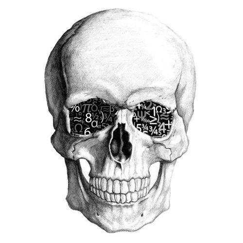
Potentially dangerous algorithms

Mathematical models and algorithms today are responsible for making important decisions affecting our daily lives, moreover, they themselves control our world.

Without higher mathematics, we would have lost Shore’s algorithm for factoring integers in quantum computers, the Yang-Mills gauge theory for building the Standard Model in particle physics, the Radon integral transform for medical and geophysical tomography, epidemiology models, insurance risk analyzes, and stochastic pricing models financial derivatives, RSA encryption, Navier-Stokes differential equations to predict changes in fluid motion and the entire climate, all developments from the theory of automatic control to methods for finding optimal solutions and a million other things that we don’t even think about.

Mathematics is at the heart of civilization. It is even more interesting to learn that since the very birth of this cornerstone it contains errors. Sometimes the mistakes of mathematics remain invisible for millennia; Sometimes they arise spontaneously and quickly spread, penetrating into our code. A typo in the equation leads to a catastrophe, but the equation itself can be potentially dangerous.

We perceive mistakes as something alien, but what if our life is built around them?

How to prove proof

Alex Bellos in his book “Beauty in the Square” discusses whether it is possible to trust computers and mathematics at all by the example of the four-color theorem. This theorem states that any map located on a sphere can be colored with no more than four different colors (colors) so that any two regions with a common part of the border are colored with different colors. At the same time, regions can be both simply connected and multiply connected (they can contain “holes”), and a common part of the border means a part of a line, that is, the joints of several areas at one point are not considered a common border for them. The theorem was formulated by Francis Guthrie in 1852 and had no proof for a long time.

In 1976, Kenneth Appel and Wolfgang Hacken of the University of Illinois used a supercomputer to check through all possible map configurations. The first step of the proof was to demonstrate that there is a certain set of 1936 maps, none of which can contain a smaller map that would disprove the theorem. The authors proved this property for each of the 1936 maps. After that, it was concluded that the smallest counterexample to the theorem does not exist, because otherwise it had to contain any of these 1936 cards, which is not.

For a long time, no one could prove the proof of a computer — too much computation was carried out to be able to check them all. From the point of view of "pure" mathematics, it was difficult to accept such a solution to the problem - it contradicted the standard of proof of theorems used since the time of Euclid. In addition, mathematicians suggested that the program could have errors. And there were indeed errors in the code.

In 2004, George Gontier from Microsoft’s research lab rechecked the evidence using the Coq v7.3.1 program using Gallina’s own functional programming language. Mathematicians asked the following question: is there any evidence that the program-checker does not contain errors? There is no complete confidence in this, however, the program has been repeatedly tested when performing many other tasks. As a result, specialized software that helps mathematicians contains tens of thousands of formal proofs.

Despite all the errors found, the proof of the four-color theorem is one of the most thoroughly verified in mathematics.

Random numbers and cryptography

Computers made it possible to significantly advance mathematics, but most importantly, they allowed to make commercially successful products out of seemingly beautiful, but “useless” theorems. One of the main achievements of computer mathematics is working with random number generators.

The problem of finding random numbers is interestingly addressed in the book of Bellos “Alex in the land of numbers. An extraordinary journey into the magical world of mathematics. ” The number π has long been considered a good example of chance. Of course, there are some sequences in infinite number. So on 17 387 594 880th place after the comma you can find the consecutive numbers 0123456789. However, this sequence is just an accident - as the experiment with a coin toss shows, contradicting intuition long sequences are more likely the norm.

Pi figures may behave as if they were random, but in fact they are predetermined. For example, if the digits in the number π were random, then the chance that the first digit after the decimal point would be equal to 1 would be equal to only 10%. However, we know with absolute certainty that there is 1; π is not accidental.

In fact, finding an accident in the surrounding phenomena is difficult. Tossing a coin randomly only because we do not think about exactly how it will land, but considering the exact speed, angle of tossing, air density and all the other essential physical parameters of the process, we can accurately calculate which side it will fall.

Translating the questions of mathematics into the plane of physics one can achieve amazing results. In 1969, mathematician Edward Thorp found out (in fact, he had been working on this issue for more than 10 years) that the casino’s desire to reduce the systematic deviation from the ideal random randomly leads to the fact that it is easier to predict the motion of the ball. The fact is that when adjusting the axis of the wheel, sometimes it is tilted - a slope of 0.2 degrees is sufficient so that a sufficiently large area appears on the funnel-like surface from which the ball never jumps onto the wheel. Using this information, you can bring the expected payoff to 0.44 of the bet.

The randomness of a number means that, among other things, it is impossible to guess the next value or the previous value of this number, even based on the knowledge of all the obsolete previous values. This can be achieved by a pseudo-random number generator (PRNG) only if it is based on the principles of robust cryptography mixed with a sufficient amount of entropy, or truly random information.

Based on pure mathematics, it is possible to make a PRNG generator with very high resistance. For example, the Blum-Blum-Shub algorithm (authors of the Blum and Michael Shub couple algorithm) has high cryptographic strength, based on the estimated complexity of factorizing integers. The algorithm is mathematically beautiful:

$$

$$X_ {n + 1} = X_ {2} ^ {n} mod M,$$

where M = pq is the product of two large primes p and q. At each step of the algorithm, the output data is obtained from X _n by taking either a parity check bit or one or more least significant bits X _n .

Some mathematicians consider the algorithm BSH and the like to be potentially dangerous, since the problem of factoring integers may not be as difficult as expected, and the output of the algorithm will be numbers that can be identified with a sufficient amount of computation. When using a fast quantum algorithm for factoring, a huge space of opportunities to search for vulnerabilities of crypto-resistant encryption will be achieved. There is no need to go far for examples. The once strong DES algorithm is now considered insufficient for many applications. Some old algorithms, which everyone thought required a billion years of computational time, can now be hacked in a few hours (MD4, MD5, SHA1, DES, and other algorithms).

In the Fortuna family of crypto-resistant generators (used in FreeBSD, OpenBSD, Mac OS X, etc.), the generator receives pseudo-random data through encryption of consecutive positive integers. The initial key becomes the initial number, and after each request the key is updated: the algorithm generates 256 bits of pseudo-random data using the old key and uses the resulting value as a new key. In addition, a block cipher in counter mode produces non-repeating 16-byte blocks with a period of ^2,128 , while in true random data with such sequence lengths, the same block values ​​are likely to occur - as we saw above using the example of Pi. Therefore, to improve the statistical properties, the maximum data size that can be issued in response to one request is limited to 2 ²⁰ bytes (with such a length of the sequence, the probability of finding the same blocks in a truly random stream is of the order of ^2–97 ). Everything else is mixed with true (possibly) random data - mouse movements, keystroke times, hard drive responses, sound card noise, and so on.

However, mathematicians even in such sets of random numbers suspect the presence of template sequences and suggest the use of unpredictable physical phenomena, such as radioactive decay and cosmic radiation.

The occurrence of errors

Sometimes all levels of protection are not enough if the programmer allows an annoying bug. An error in any step of creating a program can undermine the security of the entire system.

if ((err = SSLHashSHA1.update(...)) != 0) goto fail; goto fail; /* BUG */ if ((err = SSLHashSHA1.final(...)) != 0) goto fail; err = sslRawVerif(...); … fail: … return err; 

Classic SSL / TLS error from 2014. The additional goto statement causes iOS and Mac devices to accept invalid certificates, which makes them susceptible to MITM attacks. The developer accidentally added one redundant goto instruction, possibly via ctrl + c / ctrl + v, giving the opportunity to bypass all certificate checks for SSL / TLS connections. This error has existed for more than a year, during which millions of devices were subject to MITM attacks. Ironically, in the same year, a more serious “goto” error was detected in the GnuTLS certificate verification code. And the error existed for more than ten years.

Simple typos are sometimes unexpectedly difficult to see. Fortunately, this is exactly the mistake that can now be fixed by early tests. However, searching for more complex errors will always require more time than there is. Ultimately, the program may be more adapted to pass the tests, rather than to perform the rest of its specification.

From the point of view of mathematics, even the right equation, which gives the correct result, may contain an error that has far-reaching consequences. This idea is well illustrated by the Black-Scholes equation, which became the mathematical basis of trade and led banks to several world crises. The beautiful, correct equation did not take into account only one parameter - randomness.

The option pricing model formula was first derived by Fisher Black and Myron Scholes in 1973. An option is a contract in which the buyer of a product or security (the so-called underlying asset) is given the right (but not the obligation) to make a purchase or sale of this asset at a predetermined price at a time specified in the contract.

The model determining the theoretical price of European options implied that if the underlying asset is traded on the market, then the price of the option on it is implicitly already established by the market itself. According to the Black-Scholes model, the key element in determining the value of an option is the expected volatility (price variability) of the underlying asset. Depending on the asset's fluctuation, its price increases or decreases, which directly proportional affects the value of the option. Thus, if you know the value of the option, you can determine the level of volatility expected by the market.

The equation looks like this:

$$

$$C (S, t) = SN (d_ {1}) - Ke ^ {- r (Tt)} N (d_ {2}), \\ d_ {1} = \ frac {ln (S / K) + (r + \ sigma ^ {2} / 2) (Tt)} {\ sigma \ sqrt {Tt}} \\ d_ {2} = d_ {1} - \ sigma \ sqrt {Tt}$$

C (S, t) - the current value of the option at time t before the expiration of the option;
S - the current price of the underlying stock;
N (x) is the probability that the deviation will be less in the conditions of the standard normal distribution (and thus limit the range of values ​​for the function of the standard normal distribution);
K - option exercise price;
r - risk-free interest rate;
Tt - time before the expiration of the option (the period of the option);
σ is the volatility (square root of the variance) of the basic stock.

The equation relates the recommended price to four other values. Three can be measured directly: the time, the price of the asset at which the option is secured, and the risk-free interest rate. The fourth value is the asset volatility. This is an indicator of how volatile its market value is. The equation assumes that the asset volatility remains unchanged for the duration of the option, but this assumption turns out to be erroneous. Volatility can be estimated by statistical analysis of price movements, but it cannot be measured in an accurate, reliable way, and the estimates may not correspond to reality.

This model dates back to 1900, when the French mathematician Louis Bachelier suggested in the doctoral dissertation that the stock market fluctuations could be modeled by a random process known as the Brownian motion. At each time point, the stock price increases or decreases, and the model assumes fixed probabilities for these events. They may be equally likely or more likely than others. Their position corresponds to the stock price, moving up or down at random. The most important statistical features of the Brownian motion are its mean and standard deviation. The average is the short-term average price, which usually drifts up or down in a certain direction. The standard deviation can be considered as the average value by which the price differs from the average calculated using the standard statistical formula. For stock prices, this is called volatility, and it measures how volatile the price is.

The Black-Scholes equation made it possible to rationally evaluate a financial contract even before it began through partial differential equations expressing the rate of price change in terms of the rate of change of various other quantities. The problem of the formula turned out to be the possibility of its modification for various cases. In practice, banks use even more complex formulas, the risk assessment of which is becoming increasingly opaque. Companies hire mathematically talented analysts to develop similar formulas and get solutions that are irrelevant if market conditions change.

The model was based on the theory of arbitration pricing, in which both drift and volatility are constant. This assumption is common in financial theory, but it is often wrong for real markets - yes, this is a black-swan that has become sick of teeth. Unforeseen changes in market volatility led to consequences that it was impossible to predict using formulas. The 1998 crisis showed that a strong change in volatility happens more often than expected. The 2008 crisis demonstrated how many banks collapsed due to a shortage of liquid assets caused by an inaccurate risk assessment using non-random formulas.

The Black-Scholes equation has its roots in mathematical physics, where the quantities are infinitely divisible, time flows continuously, and the variables smoothly change. Such models may be incompatible with real life.

Original computational problems

Adequate risk assessment is crucial in predicting errors. If we calculate the risk of exposure to a giant asteroid that will kill all of humanity, the error, meaning that the asteroid actually kills humanity twice, does not matter. However, the mirror error - an asteroid that actually kills half of humanity - is of great importance!

Where is the difference between two events with an incredible calculation of the asteroid's flight, errors of the first kind (false positives) and errors of the second kind (false negatives) are shown - the key concepts of the problems of testing statistical hypotheses.

An error of the first kind is often called a false alarm, a false alarm, or a false positive response — for example, a blood test showed the presence of the disease, although in reality the person is healthy. The word “positive” in this case is not related to the desirability or undesirability of the event itself.

The magnitude of the errors of the first kind can be calculated by the formula:

$$

$$P1 = 2 * \ int_ {a} ^ {d} F (x) * dx * \ int _ {- \ infty} ^ {p} F (\ Delta) * d \ Delta,$$

Where
F (x) is the distribution function of the values ​​of the measured value;
a, d - boundaries of the interval in which there is a probability of the occurrence of errors of the first kind;
F (Δ) is the distribution function of the actual values ​​of the error of measuring instruments;
-∞, p - boundaries of the interval in which the error of measuring instruments does not prevent the occurrence of an error of the first kind.

An error of the second kind is called a pass of an event or a false-negative actuation - a person is sick, but a blood test did not show this.

The magnitude of the error of the second kind is calculated by the formula:

$$

$$P2 = 2 * \ int_ {c} ^ {a} F (x) * dx * \ int_ {p} ^ {+ \ infty} F (\ Delta) * d \ Delta,$$

Where
, a - the boundaries of the interval in which there is a probability of the occurrence of errors of the second kind;
p, + ∞ - boundaries of the interval in which the error of measuring instruments does not prevent the occurrence of an error of the second kind.

In mathematics, concepts are formed as follows:

• errors, where the theorem is still true, but the proof was incorrect, refer to the first kind;
• errors, when the theorem was false, and the proof was also incorrect, belong to the second kind.

Sometimes the occurrence of an error is associated with a change in standards of evidence. For example, when David Hilbert discovered errors in Euclidean proofs that no one had noticed before, the theorems of Euclidean geometry still remained correct, and errors arose because Hilbert was a modern mathematician, thinking in terms of formal systems (what Euclid and did not think). In turn, Hilbert himself made several other annoying mistakes: his famous list of 23 cardinal problems of mathematics contains 2 that are not correct mathematical problems (one is formulated too vaguely to understand whether it is solved or not, the other, far from solution, is physical and not mathematical).

No other science can compare with mathematics in terms of the number of errors trailing throughout human history (perhaps too loud a statement and physicists will bring many arguments in favor of their victory in this dispute). One of the most annoying blunders was associated with the absence of infinitesimal numbers in the equations, which were sometimes considered as 0, and sometimes as an infinitesimal non-zero number. On the basis of incorrect calculations in the Middle Ages, theories were built which erroneously developed over the centuries.

It is unlikely that in the 21st century, people began to be born who are fundamentally different from their ancestors and all of them are geniuses. However, it seems to us that it is we who are the most intelligent and that which we have invented is the true picture of the world. But Euclid, for example, based on logic, created a scientific structure in which his contemporaries could not find a flaw. Similarly, we may not see flaws in our mathematical tools.

Irrefutable evidence suggests that a third of all articles published in mathematical journals contain errors - not only minor errors, but also incorrect theorems and proofs. And after the mathematics should recognize the presence of problems in programming. There is such a joke (with a bit of truth) that when moving from 4000 lines of Microsoft DOS code to tens of millions of lines in subsequent versions of Windows, the number of active errors increased proportionally.

Not just programs contain errors, but math programs that should check mathematicians for errors. This common problem leads to the creation of automatic verification systems for other verification systems. For example, you can see how you found an error in the popular Mathematica system when calculating the determinant of matrices with an integer record. Mathematica not only incorrectly calculates the determinant of the matrix, but also produces different results if you evaluate the same determinant twice.

Not so long ago, mathematicians didn’t approve the use of computers at all - the need to avoid complex calculations always made progress in this area and led to the creation of elegant, beautiful solutions. And now mathematicians are used to using specialized software, which has closed source in its most popular versions (Mathematica, Maple and Magma).

Mathematicians are constantly wrong - this is normal

Mathematical errors are much more common in the computer industry than most people think. There are also many errors that go unnoticed.

Numbers of Mersenne, named after the mathematician Marin Mersenne, who studied their properties in the 17th century, have the form M _n = 2 ⁿ -1, where n is a natural number. Numbers of this type are interesting because some of them are prime numbers. Mersenn assumed that the numbers 2 ⁿ -1 are simple for n = 2, 3, 5, 7, 13, 17, 19, 31, 67, 127, 257 and composite for all other positive numbers n <257. Later it turned out that Mersenn made five errors: n = 67 and 257 give composite numbers, and n = 61, 89, 107 - simple.

Almost 200 years passed between the theory of Mersenne and the refutation.
The fact that the number 2 ⁶⁷ -1 is the product of two numbers 193 707 721 and 761 838 257 287 was proved in 1903 by Professor Cole. When asked how much time he had spent on factoring the number, Cole replied: "All Sundays are for three years."

Mathematicians are mistaken even in understanding the significance of their work. Professor G. X. Hardy of Cambridge, who worked on number theory, argued that if useful knowledge is defined as knowledge that can affect the material well-being of humanity, so that purely intellectual satisfaction is insignificant, then most of higher mathematics is useless. He justifies the pursuit of pure mathematics by the argument that its complete “uselessness” as a whole only means that it cannot be used to cause harm. Hardy stated that number theory is devoid of any practical applications; in fact, in our time, this theory is the basis of many programs that provide security.

Cerberus problem

The Kerberos network protocol, based on the Needham-Schroeder protocol, with some modifications, offers a mechanism for mutual authentication of the client and the server before establishing a connection between them. The protocol includes several degrees of protection, and Kerberos takes into account the fact that the initial exchange of information between the client and the server takes place in an unprotected environment, and the transmitted packets can be intercepted and modified.

The first version of the protocol was created in 1983 at the Massachusetts Institute of Technology (MIT) as part of the Athena project, whose main goal was to develop a plan for introducing computers into the MIT educational process. The project was educational, but ultimately gave the world several software products that are still in use today (for example, the X Window System ).

In 1989, the 4th version of the protocol appeared, which became publicly available. Other large projects on distributed systems (for example, AFS ) used Kerberos 4 ideas for their authentication systems. Kerberos random number generator has been widely used in various encryption systems for several years. And for ten years no one paid attention to the giant hole that allowed to get into any system that used the Kerberos module.

It was assumed that the program should choose a key at random from a huge array of numbers, but it turned out that the random number generator was chosen from a small set. For 10 years, researchers did not know that in Kerberos 4 random numbers are not random at all, and secret keys can be obtained within a few seconds.

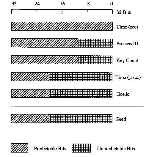
Kerberos 4 used the UNIX feature to create random 56-bit DES keys. The incorrect implementation of the algorithm used to generate pseudo-random numbers led to the fact that any sequence of key numbers had only 32 bits of entropy, of which the first 12 bits rarely changed and were predictable. As a result, Kerberos 4 only had about 220 (or about one million) possible keys.

The funny thing about this story is that Kerberos 4 has open source. The mere use of open source in itself should not lead to confidence in its correctness. Unfortunately, the availability of code available for public control led to a false understanding of security. Moreover, over time, confidence in his safety grew - it was reinforced by the belief that if problems were not yet discovered, then the probability of possible errors decreases. Trends in development, where bugs are often found in software a few days after release, as a rule, only exacerbate this common problem.

An error that means nothing

Sometimes an error does not mean that the equation or evidence must be abandoned.

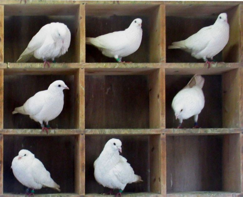
The Dirichlet principle is a famous statement formulated by the German mathematician Dirichlet in 1834, which establishes a connection between objects ("pigeons") and containers ("cells") under certain conditions, sounds like this:

If pigeons are seated in cages, and the number of pigeons is greater than the number of cells, then at least one of the cages contains more than one pigeon.

Translate into the language of mathematics:

Let at least kn + 1 pigeons sit in n cells, then at least one k + 1 pigeon sits in one of the cells.

It sounds interesting, but the most interesting thing happens in another area. In mathematical physics, the Dirichlet principle relates to potential theory and is formulated as follows: if the function u (x) is a solution to the Poisson equation

Δ u + f = 0

in the domain Ω⊂R ⁿ with the boundary condition: u = g on the boundary of Ω , then u can be found as a solution to the variational problem: find the minimum

$$

$$E [v (x)] = \ int _ {\ Omega} ^ {} (\ frac {1} {2} | \ bigtriangledown v | ^ {2} - vf) dx$$

among all twice differentiable functions v such that v = g on the boundary of Ω .

Such a beautiful and important proof of Dirichlet Lay in terms of rigorous mathematics turned out to be erroneous. A few years after his death, the mathematician Karl Weierstrass showed that the principle is not fulfilled. For this, he constructed an example in which it was impossible to find a function that minimizes the integral under given boundary conditions.

, , , .

/

, , . : . , . 2/3 : 0,6666666666666667.

7. Patriot - , 28 100. . 24- . , 1/10, , 24 .

Patriot 100 . 0,34 . 1/10 = 0,0001100110011001100110011001100… 24 0,00011001100110011001100, , 0,0000000000000000000000011001100… 0,000000095 . 0,000000095 × 100 × 60 × 60 × 10 = 0,34 .

1676 , 0,34 , .

:

(-1) ^s × M × B ^E , s — , B — , E — , M — .

, - : c/0 = ±∞ (3/0 = +∞, -3/0 = -∞, 1/∞ = 0), , , . 0/0 , NaN.

- , . FPU , , GPU CPU.

, , , , . . Sun , . 1990 Wilf-Zeilberger , , .

, /, . «» - . -1 « », . , , , . , .

, , . ,

 DO 17 I = 1, 10 

 DO17I = 1.10 

DO17I — .

Sun , , . , , Sun , , - .

« , » . 1973 , 1976 « ». : . , . . .

, . , , , .

. , . , f (x, y) = x * y x y x y. , 70- , : .

. . , , , ?

, ( ). 1990- IBM . , - 256 . , 3,7 × 10 ^-9 1,4 × 10 ^-15 . 1 20 , :

1 – (1 – 1,4,e-15)60 × 20 × 1024² = 1,8e-6

, , , . , , . - , .

1990- « » « », . , , . , , .

(. , , — , . , 21- 100 Foreign Policy . , «» — . , , , , , , , , ).

? .

, — . , : , , 9,8 / ² …

. , 9,780 /² 9,832 /², , , 9,80665 /². 9,8. , 9,8, 9,9 9,7? , 9,80000, 9,80001 9,79999?

, , , .

2008 -330 Qantas 3 , . , .

What happened? -330, , (FCPC), - (ADIRU). ADIRU Intel , . . (, , . ).

: , 1,2 . 1 — . , 1,2 . - 0,2 .

, , , . — . , .

, , — , . , - , ( ).

? — .

, , . , . . . , , , .

, , , . « » : , , , , , .

, , . , , ( SafeInt (C ++) IntegerLib (C C ++)), , .
, ? , , - « », , .

, , IT . , P ≠ NP , , , , . P NP, , . P = NP, NP- : , RSA DES/AES, .

. — 100 — . , , . , , 1000 , . , .

. , ( , ), . . - , , , , — , . ? , . , , .

, .

Probably.

( ) , , . , — , , (Steven G. Krantz, «The Proof is in the Pudding»), , .

:

How Did Software Get So Reliable Without Proof?
An Empirical Study on the Correctness of Formally Verified Distributed Systems
The misfortunes of a trio of mathematicians using Computer Algebra Systems. Can we trust in them?
The mathematical equation that caused the banks to crash
CWE-682: Incorrect Calculation
Experimental Errors and Error Analysis
Misplaced Trust: Kerberos 4 Session Keys
The Patriot Missile Failure
. «: »
. « »
Type I and Type II Errors and Their Application
Cryptographic Right Answers
Mathematical Modelling In Software Reliability