Neuroclot: Part 4 - Final Model and Product Code

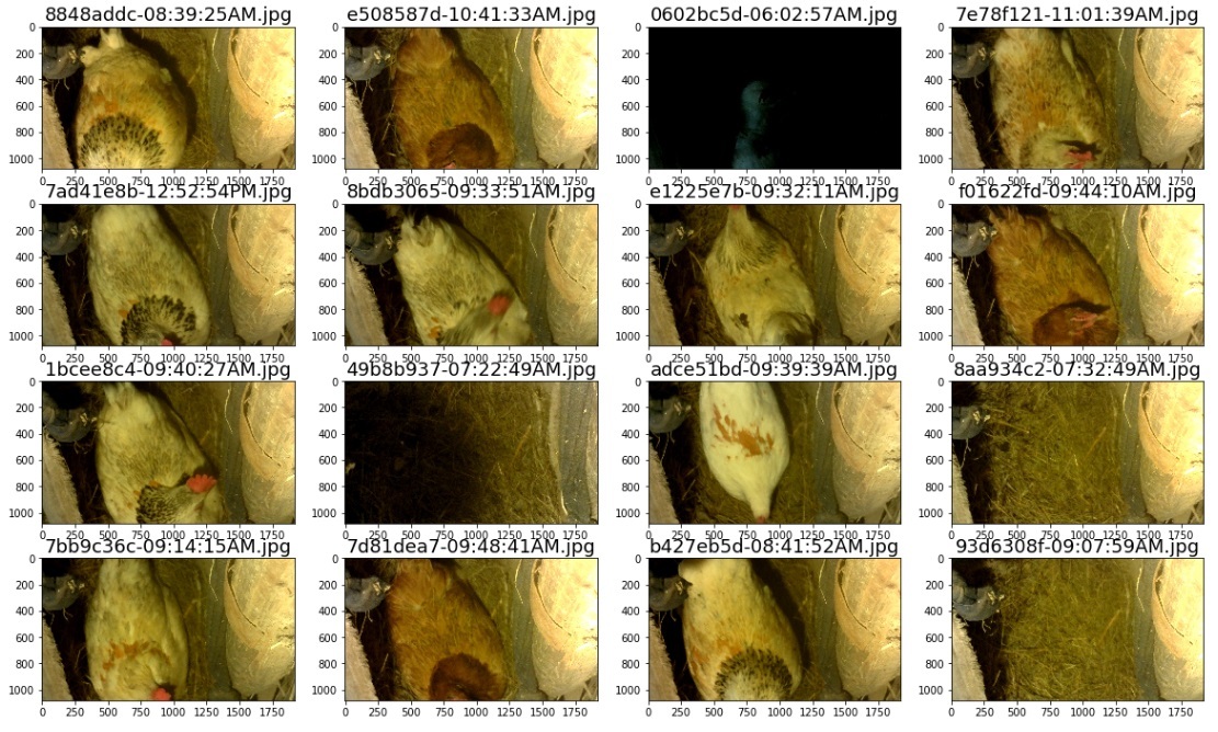
A typical day in a neurocooler - chickens often spin in the nest as well.

In order to bring, finally, the neurocooler’s project to its logical conclusion, it is necessary to produce a working model and put it on production, so that a number of conditions are met:
')

• Accuracy of predictions not less than 70-90%;
• Raspberry pi in the hen house would ideally be able to determine whether the photos belong to classes;
• It is necessary at least to learn to distinguish all chickens from each other. The maximum program is also to learn how to count eggs;

In this article we will tell you what we got in the end, what models we tried and what amusing things we caught on the road.

Articles about neurocooler

0. TL; DR

For the most impatient:

• The accuracy turned out to be about 80%;
• Dataset can be downloaded here ;
• ipynb jupyter notebook'a with all the calculations and boiler-plate code with explanations can be downloaded here , html version here ;
• Scripts for demonization and deployment on prod - here (ipynb);

1. Preludes

It also came out very opportunely, because just a few days ago this video came out, under which there is a very useful copy-paste.


From modern tools that adequately fit this goal, only convolutional neural networks come to mind. Having picked it up (by reference the recursive article about neural networks, if you want to learn) a very thorough time in neural networks, having participated in several competitions (unfortunately already closed) on Kaggle (from the open seals interested in, but there it is rather complicated) and thus mostly passing a course from fast.ai, I outlined something like this:

1. Mark a small dataset (and today you really don't need a lot of data to build a classifier);
2. Use keras to test as many architectures as possible for a maximum of 1 day;
3. If you can use unallocated photos to increase accuracy (semi-supervised approach);
4. Try to visualize the activations of the inner layers of the neural network;

2. Let's see what happened!

Layer (type) Output Shape Param # ================================================================= batch_normalization_1 (Batch (None, 700, 400, 3) 2800 _________________________________________________________________ conv2d_1 (Conv2D) (None, 698, 398, 32) 896 _________________________________________________________________ batch_normalization_2 (Batch (None, 698, 398, 32) 2792 _________________________________________________________________ max_pooling2d_1 (MaxPooling2 (None, 232, 132, 32) 0 _________________________________________________________________ conv2d_2 (Conv2D) (None, 230, 130, 64) 18496 _________________________________________________________________ batch_normalization_3 (Batch (None, 230, 130, 64) 920 _________________________________________________________________ max_pooling2d_2 (MaxPooling2 (None, 76, 43, 64) 0 _________________________________________________________________ flatten_1 (Flatten) (None, 209152) 0 _________________________________________________________________ dense_1 (Dense) (None, 200) 41830600 _________________________________________________________________ batch_normalization_4 (Batch (None, 200) 800 _________________________________________________________________ dense_2 (Dense) (None, 8) 1608 ================================================================= Total params: 41,858,912 Trainable params: 41,855,256 Non-trainable params: 3,656 _________________________________________________________________ 

The final architecture of the model in a nutshell, which gave about 80% accuracy

To begin, let's see what is happening in the hen house. To successfully make an applied project, you should always try to control the maximum part of the technological chain. It is unlikely that the project will succeed if the data comes in the form of “here you are 10 terabytes of video in terrible quality, make us a real-time video recognition model for 10,000 rubles” or “here you are 50 photos of beer labels” (humor, but these are examples , based on real ... projects, thank God not mine).

• Chickens constantly climb in the nest, just to sit or out of curiosity, especially the young;
• Young chickens (white in the photo above) - until a certain point did not lay eggs in the nest, but simply picked other people's eggs;
• Chickens have fights, but in 95% of cases the rules are observed: i) in the nest 1 chicken ii) during the stay of the chicken in the nest 10-20 unique pictures are made iii) the chicken usually completely covers the eggs with itself iv) the current view of the hens is a product several iterations of the search for the optimal location of the camera;
• On the day, about 300-400 photos are made, 5-8 eggs are laid (young chickens, due to stupidity and fear, literally rushed under the floor, then after a collection of 22 eggs was found under the floor, they began to nest in the nest);
• At night, the chickens turn off the light - they go to bed;
• About 900 photos were tagged;

Let's see how many photos came out for each class:


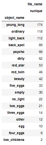
Initially, having seen such a situation, I thought that I could even distinguish photos with the number of eggs, but no. To maximize accuracy on such a small sample, you need to try to do a few things:

• Choose the right data preprocessing algorithms (it is logical that the chickens are spinning in the nest, so you can rotate the photos at least 180 degrees!);
• Choose an adequate in size and complexity model;

With preprocessing is simple - you just need to take the simplest linear model and try 5-10 combinations of parameters - with a sufficient amount of programmed sugar in Keras, this is done by substituting the parameters for such a small dataset for an hour (training 10 epochs of the model takes 50-100 seconds for 1 epoch ). Not least, this is also done for the purpose of regularization. Here is an example of one of the best practices:

 genImage = imageGeneratorSugar( featurewise_center = False, samplewise_center = False, featurewise_std_normalization = False, samplewise_std_normalization = False, rotation_range = 90, width_shift_range = 0.05, height_shift_range = 0.05, shear_range = 0.2, zoom_range = 0.2, fill_mode='constant', cval=0., horizontal_flip=False, vertical_flip=False) 

You can see the almost complete log of experiments here:

• ipynb jupyter notebook'a with all the calculations and boiler-plate code with explanations can be downloaded here , html version here ;

As for the choice of the model itself, having tested different architectures on a number of datasets, I stopped at about this model (Dropout forgot - but tests with it did not increase accuracy):

 def getTestModelNormalize(inputShapeTuple, classNumber): model = Sequential([ BatchNormalization(axis=1, input_shape = inputShapeTuple), Convolution2D(32, (3,3), activation='relu'), BatchNormalization(axis=1), MaxPooling2D((3,3)), Convolution2D(64, (3,3), activation='relu'), BatchNormalization(axis=1), MaxPooling2D((3,3)), Flatten(), Dense(200, activation='relu'), BatchNormalization(), Dense(classNumber, activation='softmax') ]) model.compile(Adam(lr=1e-4), loss='categorical_crossentropy', metrics=['accuracy']) return model 

Here is its graphic representation:



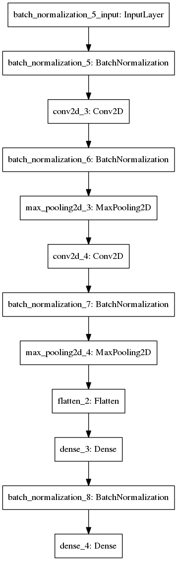
Let me explain the composition of the layers and why, in principle, almost any modern CNN looks very similar:

1. BatchNormalization - averages incoming data (subtracts the average and divides by the standard deviation), which accelerates the training of the neural network dozens of times. If you are interested for some reason, go into recursion here or here . Required to use;
2. Convolution2D - convolutional layers. In essence, they are filters so that the neural network can learn to recognize abstract images. In theory, the visualization should have been included in this article, but I didn’t master it in the end (if you don’t know how the neural network looks from inside, then here are the links for you 1 2 3 ;
3. MaxPooling2D - averaging of filter values. Mandatory after convolutional layers;
4. Dropout - essentially needed for regularization. I did not include it in this specification of the model, because I took the code from my other project and simply forgot it because of the high accuracy of the model;
5. Flatten - then insert a dense layer, otherwise it will not work;

The specification of a model with a dropout looks like this (but for some reason it did not give an increase in accuracy at first glance, as I didn’t pervert then, probably regularization and so was achieved by preprocessing photo + large photos).

 # let's try a model w dropout! def getTestModelNormalizeDropout(inputShapeTuple, classNumber): model = Sequential([ BatchNormalization(axis=1, input_shape = inputShapeTuple), Convolution2D(32, (3,3), activation='relu'), BatchNormalization(axis=1), Dropout(rate=0.3), MaxPooling2D((3,3)), Convolution2D(64, (3,3), activation='relu'), BatchNormalization(axis=1), Dropout(rate=0.1), MaxPooling2D((3,3)), Flatten(), Dense(200, activation='relu'), BatchNormalization(), Dense(classNumber, activation='softmax') ]) model.compile(Adam(lr=1e-4), loss='categorical_crossentropy', metrics=['accuracy']) return model 

Note that categorical_crossentropy is used with softmax. Adam is used as an optimizer. I will not stop why I chose them (this combination is essentially a standard), but you can read here and see 1 , 2 and 3 here .

The process of finding the optimal model looks like this:

1. We try different ways to pre-process data with the simplest model (all of a sudden the weight of the simplest dense model of 3 layers weighs a few gigabytes for large photos, which is not very good) and choose the optimal one;
2. We try different architectures of convolutional (or any other) neural networks, choose the optimal one;
3. When a significant benchmark is reached (50% + accuracy, 75% accuracy - choose from the task, the more classes, the softer the benchmark should be) - you need to analyze what model photos and which classes have problems with;
4. Ensembles and fine-tuning of the outer layers of large neural network architectures - optional - if you want to win the competition;
5. You can try to mix in your sample 20-30% of photos from the test, validation, or simply unpartitioned part of the dataset (semi-supervised, the code works, but I was the one who constantly died in this task, I scored);
6. Repeat to infinity;

 42/42 [==============================] - 87s - loss: 2.4055 - acc: 0.2783 - val_loss: 4.7899 - val_acc: 0.1771 Epoch 2/15 42/42 [==============================] - 90s - loss: 1.7039 - acc: 0.4049 - val_loss: 2.4489 - val_acc: 0.2011 Epoch 3/15 42/42 [==============================] - 90s - loss: 1.4435 - acc: 0.4827 - val_loss: 2.1080 - val_acc: 0.2402 Epoch 4/15 42/42 [==============================] - 90s - loss: 1.2525 - acc: 0.5311 - val_loss: 2.4556 - val_acc: 0.2179 Epoch 5/15 42/42 [==============================] - 85s - loss: 1.2024 - acc: 0.5549 - val_loss: 2.2180 - val_acc: 0.1955 Epoch 6/15 42/42 [==============================] - 84s - loss: 1.0820 - acc: 0.5858 - val_loss: 1.8620 - val_acc: 0.2849 Epoch 7/15 42/42 [==============================] - 84s - loss: 0.9475 - acc: 0.6535 - val_loss: 2.1256 - val_acc: 0.1955 Epoch 8/15 42/42 [==============================] - 84s - loss: 0.9283 - acc: 0.6665 - val_loss: 1.2578 - val_acc: 0.5642 Epoch 9/15 42/42 [==============================] - 84s - loss: 0.9238 - acc: 0.6792 - val_loss: 1.1639 - val_acc: 0.5698 Epoch 10/15 42/42 [==============================] - 84s - loss: 0.8451 - acc: 0.6963 - val_loss: 1.4899 - val_acc: 0.4581 Epoch 11/15 42/42 [==============================] - 84s - loss: 0.8026 - acc: 0.7183 - val_loss: 0.9561 - val_acc: 0.6480 Epoch 12/15 42/42 [==============================] - 84s - loss: 0.8353 - acc: 0.7064 - val_loss: 1.0533 - val_acc: 0.6145 Epoch 13/15 42/42 [==============================] - 84s - loss: 0.7687 - acc: 0.7380 - val_loss: 0.9039 - val_acc: 0.6760 Epoch 14/15 42/42 [==============================] - 84s - loss: 0.7683 - acc: 0.7287 - val_loss: 1.0038 - val_acc: 0.6704 Epoch 15/15 42/42 [==============================] - 84s - loss: 0.7076 - acc: 0.7451 - val_loss: 0.8953 - val_acc: 0.7039 

And this is the hypnotizing progress of the indicator ...

By the way, this code snippet will help you if you want to make a semi-supervised model in keras

 # Mix iterator class for pseudo-labelling class MixIterator(object): def __init__(self, iters): self.iters = iters self.multi = type(iters) is list if self.multi: self.N = sum([it[0].N for it in self.iters]) else: self.N = sum([it.N for it in self.iters]) def reset(self): for it in self.iters: it.reset() def __iter__(self): return self def next(self, *args, **kwargs): if self.multi: nexts = [[next(it) for it in o] for o in self.iters] n0s = np.concatenate([n[0] for n in o]) n1s = np.concatenate([n[1] for n in o]) return (n0, n1) else: nexts = [next(it) for it in self.iters] n0 = np.concatenate([n[0] for n in nexts]) n1 = np.concatenate([n[1] for n in nexts]) return (n0, n1) mi = MixIterator([batches, test_batches, val_batches) bn_model.fit_generator(mi, mi.N, nb_epoch=8, validation_data=(conv_val_feat, val_labels)) 

But if you go back to our chickens, then after step 3, after analyzing the results of the model, I saw a funny pattern.

Here is the ratio of the correct predictions to the number of photos


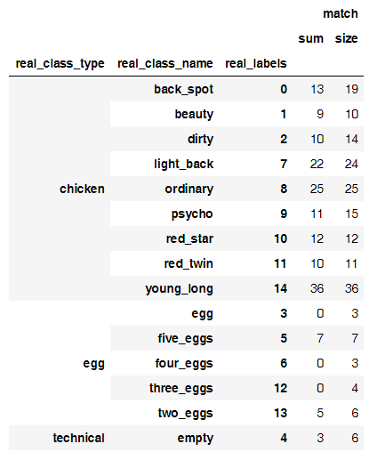
But the main source of incorrect classifications



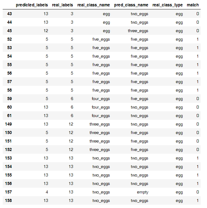
Strangely enough, on such a small sample it turned out that the neural network separates chickens from eggs well, but finds eggs with difficulty. I was able to build a separate model, which counted the eggs with 50% accuracy, but did not continue to train it, perhaps it is easier to consider eggs so .

Having placed all the eggs in one class, I ended up getting a model with about 80% accuracy on a small dataset.

3. What will go on prod?

The last stroke was deployed models for the prod. Here, of course, you need to save the weight and write a couple of functions that will spin in the daemon in the background. But here came the paste from the video at the beginning of the article.

The whole code of such a combat deployment looks like this (here tensor flow is used as a backend).

That's basically it.

 # dependencies import numpy as np import keras.models from keras.models import model_from_json from scipy.misc import imread, imresize,imshow import tensorflow as tf​​ In [3]: def init(model_file,weights_file): json_file = open(model_file,'r') loaded_model_json = json_file.read() json_file.close() loaded_model = model_from_json(loaded_model_json) #load woeights into new model loaded_model.load_weights(weights_file) print("Loaded Model from disk") #compile and evaluate loaded model loaded_model.compile(loss='categorical_crossentropy',optimizer='adam',metrics=['accuracy']) #loss,accuracy = model.evaluate(X_test,y_test) #print('loss:', loss) #print('accuracy:', accuracy) graph = tf.get_default_graph()​ return loaded_model,graph​ loaded_model,graph = init('model.json','model7_20_epochs.h5')​ In [4]: def predict(img_file, model): # here you should read the image img = imread(img_file,mode='RGB') img = imresize(img,(400,800)) #convert to a 4D tensor to feed into our model img = img.reshape(1,400,800,3) # print ("debug2") #in our computation graph with graph.as_default(): #perform the prediction out = model.predict(img) print(out) print(np.argmax(out,axis=1)) # print ("debug3") #convert the response to a string response = (np.argmax(out,axis=1)) return response In [6]: chick_dict = {0: 'back_spot', 1: 'beauty', 2: 'dirty', 3: 'egg', 4: 'empty', 5: 'light_back', 6: 'ordinary', 7: 'psycho', 8: 'red_star', 9: 'red_twin', 10: 'young_long'}​ In [7]: prediction = predict('test.jpg',loaded_model) print (chick_dict[prediction[0]]) [[ 2.34186242e-04 5.02209296e-04 5.61403576e-04 9.51264706e-03 2.03147720e-04 1.70257801e-04 4.71635815e-03 5.06504579e-03 1.84403792e-01 7.92831838e-01 1.79908809e-03]] Out [9] red_twin In [11]: import matplotlib.pyplot as plt img = imread('test.jpg',mode='RGB') plt.imshow(img) plt.show() 

Model predicts faithful chicken) Wait for the final bot, which will post faithful chickens.