Solving linear programming problems using Python
Why solve extreme problems
In practice, very often problems arise for the solution of which optimization methods are used. In everyday life, with a plurality of choices, for example, gifts for the new year, we intuitively solve the problem of minimum costs for a given quality of purchases.
Unfortunately, it is not always possible to rely on intuition. Suppose you are an employee of a commercial company and are responsible for advertising. The cost of advertising per month should not exceed 10 000 monetary units (d). A minute of radio advertising costs CU 5, and television commercials CU 90. The company intends to use radio advertising three times more often than television advertising. Practice shows that 1 minute of television advertising provides sales of 30 times more than 1 minute of radio advertising.
Your task is to determine the distribution of funds between the two types of advertising mentioned, at which the company's sales volume will be maximum. You first select the variables, namely the monthly volume in minutes on TV advertising - x1, and on radio advertising - x2. Now it is not difficult to make the following system:
30x1 + x2 - increased sales from advertising;
90x1 + 5x2 <= 10 000 - limited funds;
x2 = 3x1 - the ratio of the times of radio and television advertising.
')
Now for the time being we will forget about advertising and try to summarize the above. There may be a lot of such tasks as hardened, but they have the following common features. Obligatory is the presence of a goal-dependent linear function, in our case it is 30x1 + x2 , which, with the values of the incoming variables found, should have a single maximum value. At the same time, the condition that the incoming variables are not negative is satisfied automatically. Then follow again linear equations and inequalities in the number, depending on the presence of conditions. So we formulated one group of linear programming problems.
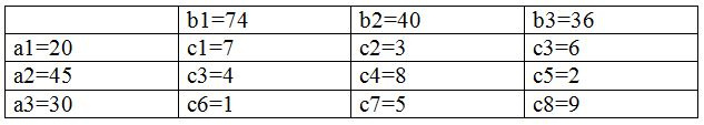
Another large group of linear programming problems, consider the example of the so-called transport problem. Suppose you are an employee of a commercial company that provides transportation services. There are suppliers of goods with warehouses in different three cities, and the volumes of homogeneous products in these warehouses are respectively equal to a1, a2, a3. There are consumers in the other three cities that need to bring goods from suppliers in volumes b1, b2, b3, respectively. Also known are the cost of shipping c1 ÷ c9 goods from suppliers to consumers, according to the table.
If x1 ... xn is the quantity of the transported cargo, then the function of the target will be the total cost of transportation:
F (x) = c1 * x1 + c2 * x2 + c3 * x3 + c4 * x4 + c5 * x5 + c6 * x6 + c7 * x7 + c8 * x8 + c9 * x9.
Conditions that are recorded. in the form of inequalities:
x1 + x2 + x3 <= 20 - you can’t take more than the supplier’s
x4 + x5 + x6 <= 45
x7 + x8 + x9 <= 30
Conditions that are recorded. in the form of equalities:
x1 + x4 + x7 = b1– as much as necessary and bring
x2 + x5 + x8 = b2
x3 + x6 + x9 = b3
Here we also need conditions for the non-negativity of the variables x, since they are not negative in meaning and the minimum of F (x) is sought. These inequalities are not given.
Now you know how to build goal functions and conditions for basic linear programming tasks. But when you read in the special literature about the geometric, simplex, artificial basis methods for solving these problems, you threw and advertising and logistics. But you can find a simple and understandable solution in Python.
Choosing Python libraries to solve common linear programming problems
For linear programming in Python, I know three specialized libraries. Consider the solution to both of the above problems in each of the libraries. In addition to the interface and optimization results, we will evaluate the performance. Since we need only a qualitative difference in speed, we will use the simplest listing for this purpose, averaging the results of each program launch.
Optimization with the pulp library [1].
Listing of the program for solving the problem “On Advertising”
from pulp import * import time start = time.time() x1 = pulp.LpVariable("x1", lowBound=0) x2 = pulp.LpVariable("x2", lowBound=0) problem = pulp.LpProblem('0',pulp.LpMaximize) problem += 30*x1 +x2, " " problem += 90*x1+ 5*x2 <= 10000, "1" problem +=x2 ==3*x1, "2" problem.solve() print (":") for variable in problem.variables(): print (variable.name, "=", variable.varValue) print (":") print (value(problem.objective)) stop = time.time() print (" :") print(stop - start) In the tenge program, the ratios already known to us for the maximum profit from advertising are 30 * x1 + x2, the cost restriction conditions marked for comparison are "1". We have not forgotten about the relationship between the times of using radio and television advertising, marked in Fox tenge as "2". The purpose of other operators is obvious. Details can be read in [1].
Results of solving an optimization problem using pulp .
Result:
x1 = 95.238095
x2 = 285.71429
Profit:
3142.85714
Time:
0.10001182556152344
As a result, we obtained the values of the times of advertising, at which the expected profit from its use will be maximum.
Optimization with the cvxopt library [2].
Program listing for solving the problem “On Advertising”.
from cvxopt.modeling import variable, op import time start = time.time() x = variable(2, 'x') z=-(30*x[0] +1*x[1])# mass1 = (90*x[0] + 5*x[1] <= 10000) #"1" mass2 = (3*x[0] -x[1] == 0) # "2" x_non_negative = (x >= 0) #"3" problem =op(z,[mass1,mass2,x_non_negative]) problem.solve(solver='glpk') problem.status print (":") print(abs(problem.objective.value()[0])) print (":") print(x.value) stop = time.time() print (" :") print(stop - start) The structure of the program is similar to the previous one, but there are two significant differences. First, the cvxopt library is set to search for the minimum of the goal function, and not the maximum. Therefore, the objective function is taken with a negative minus sign - (30 * x [0] + 1 * x [1]). The resulting negative value of it is displayed in absolute value. Secondly, the restriction on non-negativity of variables, non_negative, is introduced. Did this affect the result we now see.
Results of solving an optimization problem using cvxopt.
Profit:
3142.857142857143
Result :
[9.52e + 01]
[2.86e + 02]
Time:
0.041656494140625
There were no significant changes in comparison with the pulp library, except for the program runtime.
Optimization with the scipy library . optimiz e [3].
Program listing for solving the problem “On Advertising”.
from scipy.optimize import linprog import time start = time.time() c = [-30,-1] # A_ub = [[90,5]] #'1' b_ub = [10000]#'1' A_eq = [[3,-1]] #'2' b_eq = [0] #'2' print (linprog(c, A_ub, b_ub, A_eq, b_eq)) stop = time.time() print (" :") print(stop - start) A quick glance at the listing is enough to understand that we are dealing with a fundamentally different approach to data entry. Although the figures in the listings help clarify the principle of data organization, by comparison, I will provide explanations. The c = [-30, -1] list contains the coefficients of the target function with the opposite sign, since linprog () searches for a minimum. The matrix A_ub contains the coefficients of the variables for the conditions in the form of inequalities. For our task, this is 90x1 + 5x2 <= 10000. The values on the right side of the inequality is 1000, placed in the b_ub list. The matrix A_eq contains the coefficients of the variables for conditions in the form of equalities. For our problem, 3x1-x2 = 0 , and the zero on the right-hand side is placed on the b_eq list.
Results of solving an optimization problem using scipy. optimize.
Fun: -3142.8571428571431
message: 'Optimization terminated successfully.'
nit: 2
slack: array ([0.])
status: 0
success: True
x: array ([95.23809524, 285.71428571])
Time:
0.03020191192626953
Here the calculation results are displayed in more detail, but the results are the same as in the previous libraries.
According to the results of solving the problem “On Advertising”, an interim conclusion can be made that the use of the scipy library. optimize provides greater speed and rational form of source data. However, without the results of solving the transportation problem, it is too early to make a final conclusion.
I present a solution to the transportation problem, but without detailed explanation, since the main stages of the solution have already been described in detail.
Optimization with the pulp library.
Program listing for solving the transportation problem.
from pulp import * import time start = time.time() x1 = pulp.LpVariable("x1", lowBound=0) x2 = pulp.LpVariable("x2", lowBound=0) x3 = pulp.LpVariable("x3", lowBound=0) x4 = pulp.LpVariable("x4", lowBound=0) x5 = pulp.LpVariable("x5", lowBound=0) x6 = pulp.LpVariable("x6", lowBound=0) x7 = pulp.LpVariable("x7", lowBound=0) x8 = pulp.LpVariable("x8", lowBound=0) x9 = pulp.LpVariable("x9", lowBound=0) problem = pulp.LpProblem('0',pulp.LpMaximize) problem += -7*x1 - 3*x2 - 6* x3 - 4*x4 - 8*x5 -2* x6-1*x7- 5*x8-9* x9, " " problem +=x1 + x2 +x3<= 74,"1" problem +=x4 + x5 +x6 <= 40, "2" problem +=x7 + x8+ x9 <= 36, "3" problem +=x1+ x4+ x7 == 20, "4" problem +=x2+x5+ x8 == 45, "5" problem +=x3 + x6+x9 == 30, "6" problem.solve() print (":") for variable in problem.variables(): print (variable.name, "=", variable.varValue) print (" :") print (abs(value(problem.objective))) stop = time.time() print (" :") print(stop - start) The solution of the transportation problem requires minimization of delivery costs, therefore, the goal function is entered with a minus sign, and displayed in absolute value.
The results of solving the transport problem using pulp.
Result:
x1 = 0.0
x2 = 45.0
x3 = 0.0
x4 = 0.0
x5 = 0.0
x6 = 30.0
x7 = 20.0
x8 = 0.0
x9 = 0.0
Cost of delivery:
215.0
Time:
0.19006609916687012
Optimization with the library cvxopt .
Program listing for solving the transportation problem.
from cvxopt.modeling import variable, op import time start = time.time() x = variable(9, 'x') z=(7*x[0] + 3*x[1] +6* x[2] +4*x[3] + 8*x[4] +2* x[5]+x[6] + 5*x[7] +9* x[8]) mass1 = (x[0] + x[1] +x[2] <= 74) mass2 = (x[3] + x[4] +x[5] <= 40) mass3 = (x[6] + x[7] + x[8] <= 36) mass4 = (x[0] + x[3] + x[6] == 20) mass5 = (x[1] +x[4] + x[7] == 45) mass6 = (x[2] + x[5] + x[8] == 30) x_non_negative = (x >= 0) problem =op(z,[mass1,mass2,mass3,mass4 ,mass5,mass6, x_non_negative]) problem.solve(solver='glpk') problem.status print(":") print(x.value) print(" :") print(problem.objective.value()[0]) stop = time.time() print (" :") print(stop - start) The results of solving the transport problem using cvxopt.
Result:
[0.00e + 00]
[4.50e + 01]
[0.00e + 00]
[0.00e + 00]
[0.00e + 00]
[3.00e + 01]
[2.00e + 01]
[0.00e + 00]
[0.00e + 00]
Cost of delivery:
215.0
Time:
0.03001546859741211
Optimization with the scipy library. optimize.
Program listing for solving the transportation problem.
from scipy.optimize import linprog import time start = time.time() c = [7, 3, 6,4,8,2,1,5,9] A_ub = [[1,1,1,0,0,0,0,0,0], [0,0,0,1,1,1,0,0,0], [0,0,0,0,0,0,1,1,1]] b_ub = [74,40,36] A_eq = [[1,0,0,1,0,0,1,0,0], [0,1,0,0,1,0,0,1,0], [0,0,1,0,0,1,0,0,1]] b_eq = [20,45,30] print(linprog(c, A_ub, b_ub, A_eq, b_eq)) stop = time.time() print (" :") print(stop - start) The results of solving the transport problem using scipy optimize.
fun: 215.0
message: 'Optimization terminated successfully.'
nit: 9
slack: array ([29., 10., 16.])
status: 0
success: True
x: array ([0., 45., 0., 0., 0., 30., 20., 0., 0.])
Time:
0.009982585906982422
The analysis of the solution of two typical linear programming problems with the help of three libraries of similar purpose does not raise doubts in the choice of the scipy library. optimize, as a leader in data entry compactness and speed.
Whats new to use the scipy library. optimize when solving linear programming problems
Obtaining from the source matrix, a list for the goal function, as well as filling the A_ub inequalities matrices and A_eq equalities programmatically, will simplify the data entry work and increase the dimension of the original matrix. This allows solving real optimization problems. Let us consider how this can be done with a simple demo, which does not pretend to code ideality.
Spoiler header
import numpy as np from scipy.optimize import linprog b_ub = [74,40,36] b_eq = [20,45,30] A=np.array([[7, 3,6],[4,8,2],[1,5,9]]) m, n = A.shape c=list(np.reshape(A,n*m))# A c. A_ub= np.zeros([m,m*n]) for i in np.arange(0,m,1):# –. for j in np.arange(0,n*m,1): if i*n<=j<=n+i*n-1: A_ub [i,j]=1 A_eq= np.zeros([m,m*n]) for i in np.arange(0,m,1):# –. k=0 for j in np.arange(0,n*m,1): if j==k*n+i: A_eq [i,j]=1 k=k+1 print(linprog(c, A_ub, b_ub, A_eq, b_eq)) Now, only the matrix A itself and the right parts of the b_ub inequalities and b_ub - equalities are entered.
The result of the program is predictable.
fun: 215.0
message: 'Optimization terminated successfully.'
nit: 9
slack: array ([29., 10., 16.])
status: 0
success: True
x: array ([0., 45., 0., 0., 0., 30., 20., 0., 0.])
Private withdrawal
When solving linear programming problems, it is advisable to use the scipy.optimize library as described in the article, and to fill in the matrix of conditions programmatically. In this case, you do not need special knowledge about the methods of solving optimization problems.
Common conclusion
Recently, various Python libraries have appeared solving a similar problem. The decision on the use of a library is often subjective. Therefore, it is advisable to carry out their comparative analysis for the field of problems you are solving.
Links
Source: https://habr.com/ru/post/330648/
All Articles