We have already covered PostgreSQL's indexing mechanism and access methods interface , as well as one of the access methods, the hash index . Now let's talk about the most traditional and used index - the B-tree. The head turned out great, be patient.

Btree

Device

The btree index, also known as the B-tree, is suitable for data that can be sorted. In other words, for the data type, the operators "greater than", "greater than or equal to", "less than", "less than or equal to" and "equal" should be defined. Notice that the same data can sometimes be sorted in different ways, which brings us back to the concept of a family of operators.

As always, B-tree index records are packed into pages. In leaf pages, these records contain indexed data (keys) and links to table rows (TIDs); in the inner pages, each entry refers to the child page of the index and contains the minimum key value in this page.

B-trees have several important properties:
')

• They are balanced, that is, any sheet page separates the same number of inner pages from the root. Therefore, the search for any value takes the same time.
  
• They are very branchy, that is, each page (as a rule, 8 KB) contains many (hundreds) TIDs at once. Due to this, the depth of the B-trees is small; in practice, up to 4–5 for very large tables.
  
• The data in the index is arranged in non-decreasing order (both between the pages and within each page), and the pages of the same level are linked by a bi-directional list. Therefore, we can get an ordered set of data, simply by going through the list in one direction or the other, without returning to the root each time.
  

Here is a schematic example of an index on a single field with integer keys.



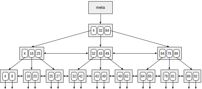
At the very beginning of the file is the metastpage, which refers to the index root. Below the root are the internal nodes; the bottom row is leaf pages. The down arrows symbolize links from leaf nodes to table rows (TIDs).

Equality Search

Consider searching for a value in a tree by the condition “ indexed-field = expression ”. Suppose we are interested in key 49.



The search starts from the root node, and we need to determine which of the child nodes to descend. By knowing the keys in the root node (4, 32, 64), we thereby understand the ranges of values ​​in the child nodes. Since 32 ≤ 49 <64, it is necessary to go down to the second child node. Then the same procedure is repeated recursively until a leaf node is reached, from which the necessary TIDs can already be obtained.

In reality, this seemingly simple procedure is complicated by a number of circumstances. For example, the index may contain non-unique keys and the same values ​​may be quite a lot so that they do not fit on one page. Continuing our example, it seems that from the internal node we should go down the link that leads from the value 49. But, as can be seen in the picture, we’ll skip one of the keys 49 in the previous leaf page. Therefore, having found the exact key equality on the inner page, we have to go down one position to the left, and then view the index records of the underlying level from left to right in search of the key of interest.

(Another difficulty is caused by the fact that during the search other processes can change the data: the tree can be rebuilt, the pages can be divided into two, etc. All algorithms are designed so that these simultaneous actions do not interfere with each other and do not require unnecessary locks. But we will not go into these details any more.)

Inequality search

When searching by the condition “ indexed-field ≤ expression ” (or “ indexed-field ≥ expression ”), first we find in the index the value by the condition of equality “ indexed-field = expression ” (if any), and then we move along the leaf pages to end in the right direction.

The figure illustrates this process for the condition n ≤ 35:



The operators “more” and “less” are supported in the same way, it is only necessary to exclude the original value found.

Search by range

When searching by the range “ expression1 ≤ indexed-field ≤ expression2 ” we find the value by the condition “ indexed-field = expression1 ”, and then we move through the leaf pages until the condition “ indexed-field ≤ expression2 ” is fulfilled. Or vice versa: we start from the second expression and move in the other direction until we reach the first.

The figure shows the process for condition 23 ≤ n ≤ 64:

Example

Let's see what the query plans look like by example. As usual, we use a demo database, and this time we take a table of aircraft. There are only nine lines in it and the scheduler will not use an index of its own free will, because the entire table is placed in one page. But we are interested in it because of clarity.

demo=# select * from aircrafts;
aircraft_code | model | range
---------------+---------------------+-------
773 | Boeing 777-300 | 11100
763 | Boeing 767-300 | 7900
SU9 | Sukhoi SuperJet-100 | 3000
320 | Airbus A320-200 | 5700
321 | Airbus A321-200 | 5600
319 | Airbus A319-100 | 6700
733 | Boeing 737-300 | 4200
CN1 | Cessna 208 Caravan | 1200
CR2 | Bombardier CRJ-200 | 2700
(9 rows)

demo=# create index on aircrafts(range);
CREATE INDEX

demo=# set enable_seqscan = off;
SET

(Or explicitly create index on aircrafts using btree (range), but by default it is the B-tree that is built.)

Equality Search:

demo=# explain(costs off) select * from aircrafts where range = 3000;
QUERY PLAN
---------------------------------------------------
Index Scan using aircrafts_range_idx on aircrafts
Index Cond: (range = 3000)
(2 rows)

Search for inequality:

demo=# explain(costs off) select * from aircrafts where range < 3000;
QUERY PLAN
---------------------------------------------------
Index Scan using aircrafts_range_idx on aircrafts
Index Cond: (range < 3000)
(2 rows)

And by range:

demo=# explain(costs off) select * from aircrafts where range between 3000 and 5000;
QUERY PLAN
-----------------------------------------------------
Index Scan using aircrafts_range_idx on aircrafts
Index Cond: ((range >= 3000) AND (range <= 5000))
(2 rows)


Sorting

It is worth emphasizing once again that with any scanning method (index, exclusively index, on a bitmap), the btree access method returns ordered data, which is clearly seen in the figures above.

Therefore, if there is an index on the table according to the sorting condition, the optimizer will take into account both possibilities: reference to the table by index and automatic retrieval of sorted data, or sequential reading of the table and subsequent sorting of the result.

The sort order

When creating an index, you can explicitly specify the sort order. For example, an index on the flight range could be created like this:

demo=# create index on aircrafts(range desc);

In this case, to the left in the tree would be greater values, and to the right - smaller values. Why this may be needed if the indexed values ​​can be passed in one direction or in the other?

The reason is multi-column indexes. Let's create an idea that will show the models of aircraft and conditional division into short, medium and long-haul vessels:

demo=# create view aircrafts_v as
select model,
case
when range < 4000 then 1
when range < 10000 then 2
else 3
end as class
from aircrafts;
CREATE VIEW

demo=# select * from aircrafts_v;
model | class
---------------------+-------
Boeing 777-300 | 3
Boeing 767-300 | 2
Sukhoi SuperJet-100 | 1
Airbus A320-200 | 2
Airbus A321-200 | 2
Airbus A319-100 | 2
Boeing 737-300 | 2
Cessna 208 Caravan | 1
Bombardier CRJ-200 | 1
(9 rows)

And create an index (using an expression):

demo=# create index on aircrafts(
(case when range < 4000 then 1 when range < 10000 then 2 else 3 end), model);
CREATE INDEX

Now we can use this index to get the data sorted by both columns in ascending order:

demo=# select class, model from aircrafts_v order by class, model;
class | model
-------+---------------------
1 | Bombardier CRJ-200
1 | Cessna 208 Caravan
1 | Sukhoi SuperJet-100
2 | Airbus A319-100
2 | Airbus A320-200
2 | Airbus A321-200
2 | Boeing 737-300
2 | Boeing 767-300
3 | Boeing 777-300
(9 rows)

demo=# explain(costs off) select class, model from aircrafts_v order by class, model;
QUERY PLAN
--------------------------------------------------------
Index Scan using aircrafts_case_model_idx on aircrafts
(1 row)

Similarly, you can execute a query with sorting in descending order:

demo=# select class, model from aircrafts_v order by class desc, model desc;
class | model
-------+---------------------
3 | Boeing 777-300
2 | Boeing 767-300
2 | Boeing 737-300
2 | Airbus A321-200
2 | Airbus A320-200
2 | Airbus A319-100
1 | Sukhoi SuperJet-100
1 | Cessna 208 Caravan
1 | Bombardier CRJ-200
(9 rows)

demo=# explain(costs off)
select class, model from aircrafts_v order by class desc, model desc;
QUERY PLAN
-----------------------------------------------------------------
Index Scan Backward using aircrafts_case_model_idx on aircrafts
(1 row)

But from this index it is impossible to obtain data sorted by one column in descending order, and the other - in ascending order. To do this, you will need to sort separately:

demo=# explain(costs off)
select class, model from aircrafts_v order by class asc , model desc ;
QUERY PLAN
-------------------------------------------------
Sort
Sort Key: (CASE ... END), aircrafts.model DESC
-> Seq Scan on aircrafts
(3 rows)

(Note that with grief, the scheduler chose to scan the table, even though the enable_seqscan = off setting was made earlier. This is because, in fact, it does not prohibit scanning the table, but only sets it beyond the limit cost - see the plan with “costs on”. )

In order for such a query to be executed using an index, the index must be constructed and sorted in the necessary order:

demo=# create index aircrafts_case_asc_model_desc_idx on aircrafts(
(case when range < 4000 then 1 when range < 10000 then 2 else 3 end) asc , model desc );
CREATE INDEX

demo=# explain(costs off)
select class, model from aircrafts_v order by class asc , model desc ;
QUERY PLAN
-----------------------------------------------------------------
Index Scan using aircrafts_case_asc_model_desc_idx on aircrafts
(1 row)


Column order

Another issue that arises when using multi-column indexes is the order of listing the columns in the index. In the case of a B-tree, this order is of great importance: the data inside the pages will be sorted first by the first field, then by the second, and so on.

The index, which we built by range intervals and models, can be represented as follows:



Of course, in fact, such a small index will fit into one root page; in the figure it is artificially distributed over several pages for clarity.

From this scheme, it is clear that the search will work effectively with such, for example, predicates, like "class = 3" (search only for the first field) or "class = 3 and model = 'Boeing 777-300'" (search by both fields ).

But the search for the predicate “model = 'Boeing 777-300'” will be much less effective: starting from the root, we cannot determine which of the child nodes to descend, so we will have to go down to everything. This does not mean that such an index can not be used in principle - the only question is efficiency. For example, if we had three classes of airplanes and a lot of models in each class, we would have to look at about a third of the index, and this could be more efficient than a full table scan. And it could not be.

But if you create an index like this:

demo=# create index on aircrafts(
model, (case when range < 4000 then 1 when range < 10000 then 2 else 3 end));
CREATE INDEX

then the order of the fields will change:



And with this index, the search by the predicate “model = 'Boeing 777-300'” will be performed efficiently, but by the predicate “class = 3” - not.

Undefined values

The btree access method indexes null values ​​and supports searching by conditions is null and is not null.

Take the table of flights, in which there are uncertain values:

demo=# create index on flights(actual_arrival);
CREATE INDEX
demo=# explain(costs off) select * from flights where actual_arrival is null;
QUERY PLAN
-------------------------------------------------------
Bitmap Heap Scan on flights
Recheck Cond: (actual_arrival IS NULL)
-> Bitmap Index Scan on flights_actual_arrival_idx
Index Cond: (actual_arrival IS NULL)
(4 rows)

Indefinite values ​​are located on one or the other edge of the leaf nodes, depending on how the index was created (nulls first or nulls last). This is important if the query is involved in sorting: the order in which the undefined values ​​are placed in the index and in the sort order must match for the index to be used.
In this example, the orders are the same, so the index can be used:

demo=# explain(costs off) select * from flights order by actual_arrival nulls last ;
QUERY PLAN
--------------------------------------------------------
Index Scan using flights_actual_arrival_idx on flights
(1 row)

And here the orders are different, and the optimizer selects a table scan and sort:

demo=# explain(costs off) select * from flights order by actual_arrival nulls first ;
QUERY PLAN
----------------------------------------
Sort
Sort Key: actual_arrival NULLS FIRST
-> Seq Scan on flights
(3 rows)

For an index to be used, you must create it so that the undefined values ​​go at the beginning:

demo=# create index flights_nulls_first_idx on flights(actual_arrival nulls first );
CREATE INDEX
demo=# explain(costs off) select * from flights order by actual_arrival nulls first ;
QUERY PLAN
-----------------------------------------------------
Index Scan using flights_nulls_first_idx on flights
(1 row)

The reason for such discrepancies, of course, is that undefined values ​​are not sortable: the result of comparing an undefined value with any other value is undefined:

demo=# \pset null NULL
Null display is "NULL".
demo=# select null < 42;
?column?
----------
NULL
(1 row)

This goes against the essence of the B-tree and does not fit into the overall scheme. But indefinite values ​​play such an important role in databases that they have to make exceptions all the time.

The fact that undefined values ​​are indexed is the ability to use an index, even if no conditions are imposed on the table at all (since the index is guaranteed to contain information about all the rows in the table). This may make sense if the query needs to organize the data and the index provides the desired order. Then the scheduler may prefer index access to save on separate sorting.

Properties

Let's look at the properties of the btree access method (requests were cited earlier ).

amname | name | pg_indexam_has_property
--------+---------------+-------------------------
btree | can_order | t
btree | can_unique | t
btree | can_multi_col | t
btree | can_exclude | t

As we have seen, a B-tree can organize data and maintains uniqueness — and this is the only access method that provides such properties. Multiple column indices are also allowed; but other methods can do this (although not all). We’ll talk about support for the limitations of exclude, not without reason, next time.

name | pg_index_has_property
---------------+-----------------------
clusterable | t
index_scan | t
bitmap_scan | t
backward_scan | t

The b-tree access method supports both ways of getting values: both index scanning and bitmap scanning. And, as we have seen, can bypass the tree as "forward", and in the opposite direction.

name | pg_index_column_has_property
--------------------+------------------------------
asc | t
desc | f
nulls_first | f
nulls_last | t
orderable | t
distance_orderable | f
returnable | t
search_array | t
search_nulls | t

The first four properties of this level talk about how the values ​​of this particular column are ordered. In this example, the values ​​are sorted in ascending order (asc), and the undefined values ​​are at the end (nulls_last). But, as we have seen, there may be other combinations.

The search_array property indicates that the index supports such constructs:

demo=# explain(costs off)
select * from aircrafts where aircraft_code in ('733','763','773');
QUERY PLAN
-----------------------------------------------------------------
Index Scan using aircrafts_pkey on aircrafts
Index Cond: (aircraft_code = ANY ('{733,763,773}'::bpchar[]))
(2 rows)

The returnable property indicates support for index scans only - which is logical, because indexed values ​​themselves store indexed values ​​(as opposed to a hash index, for example). It is appropriate to say a few words about the features of the covering indices based on the B-tree.

Unique indexes with extra columns

As we said earlier , the covering is an index that contains all the values ​​required in the query; at the same time, reference to the table itself is no longer required (almost). Including the cover may be a unique index.

But suppose we want to add to the unique index the additional columns needed in the query. The values ​​of the new composite key may not already be unique, and then you will need to have two indices for almost the same columns: one unique (to support integrity constraints) and one more non-unique (as a cover). This, of course, is ineffective.

In our company, Anastasia Lubennikova lubennikovaav refined the btree method so that you can include additional - non-unique - columns in the unique index. We hope that this patch will be accepted by the community and will be included in PostgreSQL, but this will not happen in version 10. While the patch is available in Postgres Pro Standard 9.5+, and this is how it looks.

Take the booking table:

demo=# \d bookings
Table "bookings.bookings"
Column | Type | Modifiers
--------------+--------------------------+-----------
book_ref | character(6) | not null
book_date | timestamp with time zone | not null
total_amount | numeric(10,2) | not null
Indexes:
"bookings_pkey" PRIMARY KEY, btree (book_ref)
Referenced by:
TABLE "tickets" CONSTRAINT "tickets_book_ref_fkey" FOREIGN KEY (book_ref) REFERENCES bookings(book_ref)

In it, the primary key (book_ref, reservation code) is supported by the usual btree-index. Create a new unique index with an additional column:

demo=# create unique index bookings_pkey2 on bookings(book_ref) include (book_date) ;
CREATE INDEX

Now we will replace the existing index with a new one (in a transaction so that all changes take effect at the same time):

demo=# begin;
BEGIN
demo=# alter table bookings drop constraint bookings_pkey cascade;
NOTICE: drop cascades to constraint tickets_book_ref_fkey on table tickets
ALTER TABLE
demo=# alter table bookings add primary key using index bookings_pkey2 ;
ALTER TABLE
demo=# alter table tickets add foreign key (book_ref) references bookings (book_ref);
ALTER TABLE
demo=# commit;
COMMIT

Here's what happened:

demo=# \d bookings
Table "bookings.bookings"
Column | Type | Modifiers
--------------+--------------------------+-----------
book_ref | character(6) | not null
book_date | timestamp with time zone | not null
total_amount | numeric(10,2) | not null
Indexes:
"bookings_pkey2" PRIMARY KEY, btree (book_ref) INCLUDE (book_date)
Referenced by:
TABLE "tickets" CONSTRAINT "tickets_book_ref_fkey" FOREIGN KEY (book_ref) REFERENCES bookings(book_ref)

Now the same index works as a unique one, and acts as a covering for such, for example, query:

demo=# explain(costs off)
select book_ref, book_date from bookings where book_ref = '059FC4';
QUERY PLAN
--------------------------------------------------
Index Only Scan using bookings_pkey2 on bookings
Index Cond: (book_ref = '059FC4'::bpchar)
(2 rows)


Create index

A well-known, but no less important fact from this: it is better to load a large amount of data into a table without indexes, and create the necessary indexes after. This is not only faster, but the index itself will most likely get smaller.

The fact is that when creating a btree-index, a more efficient procedure is used than progressively inserting values ​​into a tree. Roughly speaking, all the data in the table is sorted and sheet pages of the index are formed; then internal pages are “built up” on this basis until the whole pyramid converges to the root.

The speed of this process depends on the size of available RAM, which is limited by the maintenance_work_mem parameter, so an increase in the value can lead to acceleration. In the case of unique indexes, in addition to maintenance_work_mem, memory is also allocated with the size of work_mem.

Comparison semantics

Last time we talked about the fact that PostgreSQL needs to know which hash functions to call for values ​​of different types, and that such a correspondence is stored in the hash access method. In the same way, the system needs to understand how to order values ​​- it is necessary for sorting, grouping (sometimes), merge joins, etc. PostgreSQL does not bind to operator names (such as>, <, =), because the user may well define your data type and name the corresponding operators in some other way. Instead, the names of the operators are determined by the family of operators associated with the btree access method.

For example, here are some comparison operators used in the bool_ops family:

postgres=# select amop.amopopr::regoperator as opfamily_operator,
amop.amopstrategy
from pg_am am,
pg_opfamily opf,
pg_amop amop
where opf.opfmethod = am.oid
and amop.amopfamily = opf.oid
and am.amname = 'btree'
and opf.opfname = 'bool_ops'
order by amopstrategy;

opfamily_operator | amopstrategy
---------------------+--------------
<(boolean,boolean) | 1
<=(boolean,boolean) | 2
=(boolean,boolean) | 3
>=(boolean,boolean) | 4
>(boolean,boolean) | 5
(5 rows)

Here we see five comparison operators, but, as was said, should not be guided by their names. To understand which comparison is implemented by which operator, the concept of strategy is introduced . For btree, five strategies are defined that define the semantics of operators:

• 1 - less;
• 2 - less or equal;
• 3 equals;
• 4 - more or equal;
• 5 - more.

Some families may contain several operators implementing one strategy. For example, here are some operators in the integer_ops family for strategy 1:

postgres=# select amop.amopopr::regoperator as opfamily_operator
from pg_am am,
pg_opfamily opf,
pg_amop amop
where opf.opfmethod = am.oid
and amop.amopfamily = opf.oid
and am.amname = 'btree'
and opf.opfname = 'integer_ops'
and amop.amopstrategy = 1
order by opfamily_operator;

opfamily_operator
----------------------
<(integer,bigint)
<(smallint,smallint)
<(integer,integer)
<(bigint,bigint)
<(bigint,integer)
<(smallint,integer)
<(integer,smallint)
<(smallint,bigint)
<(bigint,smallint)
(9 rows)

Due to this, the optimizer has the ability to compare the values ​​of different types belonging to the same family without resorting to casting.

Index support for new data type

The documentation has an example of creating a new data type for complex numbers, and a class of operators for sorting values ​​of this type. This example uses the C language, which is absolutely justified when speed is important. But nothing prevents you from doing the same experiment on pure SQL, just to try and better understand the semantics of the comparison.

Create a new composite type with two fields: the real and imaginary parts.

postgres=# create type complex as (re float, im float);
CREATE TYPE

You can create a table with a new type field and add some values ​​to it:

postgres=# create table numbers(x complex);
CREATE TABLE
postgres=# insert into numbers values ((0.0, 10.0)), ((1.0, 3.0)), ((1.0, 1.0));
INSERT 0 3

Now the question arises: how to order complex numbers if, in the mathematical sense, the order relation is not defined for them?

As it turns out, comparison operations are already defined for us:

postgres=# select * from numbers order by x;
x
--------
(0,10)
(1,1)
(1,3)
(3 rows)

By default, the composite type is sorted by component: first, the first fields are compared, then the second, and so on, just like text strings are compared character by character. But you can define a different order. For example, complex numbers can be considered as vectors and ordered by modulo (by length), which is calculated as the root of the sum of squares of coordinates (Pythagorean theorem). To determine this order, create an auxiliary function to calculate the module:

postgres=# create function modulus(a complex) returns float as $$
select sqrt(a.re*a.re + a.im*a.im);
$$ immutable language sql;
CREATE FUNCTION

And with its help we will methodically define the functions for all five comparison operations:

postgres=# create function complex_lt(a complex, b complex) returns boolean as $$
select modulus(a) < modulus(b);
$$ immutable language sql;
CREATE FUNCTION
postgres=# create function complex_le(a complex, b complex) returns boolean as $$
select modulus(a) <= modulus(b);
$$ immutable language sql;
CREATE FUNCTION
postgres=# create function complex_eq(a complex, b complex) returns boolean as $$
select modulus(a) = modulus(b);
$$ immutable language sql;
CREATE FUNCTION
postgres=# create function complex_ge(a complex, b complex) returns boolean as $$
select modulus(a) >= modulus(b);
$$ immutable language sql;
CREATE FUNCTION
postgres=# create function complex_gt(a complex, b complex) returns boolean as $$
select modulus(a) > modulus(b);
$$ immutable language sql;
CREATE FUNCTION

And create the appropriate operators. To show that they are not required to be called ">", "<", and so on, we give them "strange" names.

postgres=# create operator #<#(leftarg=complex, rightarg=complex, procedure=complex_lt);
CREATE OPERATOR
postgres=# create operator #<=#(leftarg=complex, rightarg=complex, procedure=complex_le);
CREATE OPERATOR
postgres=# create operator #=#(leftarg=complex, rightarg=complex, procedure=complex_eq);
CREATE OPERATOR
postgres=# create operator #>=#(leftarg=complex, rightarg=complex, procedure=complex_ge);
CREATE OPERATOR
postgres=# create operator #>#(leftarg=complex, rightarg=complex, procedure=complex_gt);
CREATE OPERATOR

At this stage, you can already compare the numbers:

postgres=# select (1.0,1.0)::complex #<# (1.0,3.0)::complex;
?column?
----------
t
(1 row)

In addition to the five operators, the btree access method requires you to define another (redundant but convenient) function: it must return -1, 0 or 1 if the first value is less, equal or greater than the second. Such an auxiliary function is called support; other access methods may require the creation of other support functions.

postgres=# create function complex_cmp(a complex, b complex) returns integer as $$
select case when modulus(a) < modulus(b) then -1
when modulus(a) > modulus(b) then 1
else 0
end;
$$ language sql;
CREATE FUNCTION

Now we are ready to create a class of operators (and the family of the same name will be created automatically):

postgresx=# create operator class complex_ops
default for type complex
using btree as
operator 1 #<#,
operator 2 #<=#,
operator 3 #=#,
operator 4 #>=#,
operator 5 #>#,
function 1 complex_cmp(complex,complex);
CREATE OPERATOR CLASS

Now sorting works as we wanted:

postgres=# select * from numbers order by x;
x
--------
(1,1)
(1,3)
(0,10)
(3 rows)

And, of course, it will be supported by the btree index.

For the sake of completeness, the reference functions can be seen with the following query:

postgres=# select amp.amprocnum,
amp.amproc,
amp.amproclefttype::regtype,
amp.amprocrighttype::regtype
from pg_opfamily opf,
pg_am am,
pg_amproc amp
where opf.opfname = 'complex_ops'
and opf.opfmethod = am.oid
and am.amname = 'btree'
and amp.amprocfamily = opf.oid;

amprocnum | amproc | amproclefttype | amprocrighttype
-----------+-------------+----------------+-----------------
1 | complex_cmp | complex | complex
(1 row)


Insides

The internal structure of a B-tree can be studied using the pageinspect extension.

demo=# create extension pageinspect;
CREATE EXTENSION

Index index:

demo=# select * from bt_metap('ticket_flights_pkey');
magic | version | root | level | fastroot | fastlevel
--------+---------+------+-------+----------+-----------
340322 | 2 | 164 | 2 | 164 | 2
(1 row)

The most interesting thing here is the depth of the index (level): placing the index in two columns for a table with a million rows required only 2 levels (not counting the root).

Statistical information about block 164 (root):

demo=# select type, live_items, dead_items, avg_item_size, page_size, free_size
from bt_page_stats('ticket_flights_pkey',164);
type | live_items | dead_items | avg_item_size | page_size | free_size
------+------------+------------+---------------+-----------+-----------
r | 33 | 0 | 31 | 8192 | 6984
(1 row)

And the data itself in the block (in the data field, which is sacrificed for the width of the screen, is the value of the index key in binary form):

demo=# select itemoffset, ctid, itemlen, left(data,56) as data
from bt_page_items('ticket_flights_pkey',164) limit 5;
itemoffset | ctid | itemlen | data
------------+---------+---------+----------------------------------------------------------
1 | (3,1) | 8 |
2 | (163,1) | 32 | 1d 30 30 30 35 34 33 32 33 30 35 37 37 31 00 00 ff 5f 00
3 | (323,1) | 32 | 1d 30 30 30 35 34 33 32 34 32 33 36 36 32 00 00 4f 78 00
4 | (482,1) | 32 | 1d 30 30 30 35 34 33 32 35 33 30 38 39 33 00 00 4d 1e 00
5 | (641,1) | 32 | 1d 30 30 30 35 34 33 32 36 35 35 37 38 35 00 00 2b 09 00
(5 rows)

The first element is technical in nature and sets the upper limit of the key value of all elements of the block (implementation detail, about which we did not speak), and the actual data begins with the second element. It can be seen that the block 163 is the leftmost daughter node, then block 323 and so on. Which, in turn, can also be studied using the same functions.

Further, by a good tradition, it makes sense to read the documentation, the README and the source code.

And one more potentially useful extension: amcheck , which will be part of PostgreSQL 10, and for earlier versions you can take it on github . This extension checks the logical consistency of data in B-trees and allows for early detection of damage.

Continued .