Fast data recovery. How will LRC help us?

In the modern world, there is an exponential growth in data volumes. Storage vendors face a whole range of tasks associated with colossal amounts of information. Among them - the protection of user data from loss and the fastest possible data recovery in the event of a server or disk failure.

Our article will consider the task of quick reconstruction. It would seem that the best solution for data protection is replication, but the volume of service information in this scenario is 100% or more. It is not always possible to select such a volume. Therefore, a compromise must be sought between redundancy and speed of recovery.

A well-known approach that provides less overhead is local parity codes (LRC) and regeneration codes . These solutions work for both distributed systems and local disk arrays.

In this article, we will look at the specifics of using LRC codes for disk arrays and offer scenarios for accelerated recovery of failed disk data.
')
We conducted performance testing simultaneously for both LRC and regenerating codes, but we will describe the latter in more detail in one of the following articles.

Data availability

RAID technology (Redundant Array of Independent Disks) is used in data storage systems to provide high speed data access and fault tolerance. High speed is achieved by parallelizing the processes of reading and writing data to disks, and fault tolerance is achieved through the use of error-correcting coding.

Over time, the requirements for storage capacity and reliability have increased. This led to the emergence of new RAID levels (RAID-1 ... 6, RAID-50, RAID-60, RAID-5E, etc.) and the use of different classes of error-correcting codes, like MDS (Maximum distance separable - codes with maximum code distance) and non-MDS.

We consider how the placement of data with a certain encoding method affects the speed of recovery of a failed disk, and, as a result, the availability of data on the disk array.

Availability is the probability that the system will be available upon request. High availability is achieved, in particular, by coding, i.e. Part of the system disk space is not allocated for user data, but for storage of checksums. In the event of a system disk failure, lost data can be recovered using these checksums — thereby ensuring data availability. As a rule, availability is calculated by the formula:

A v a i l a b i l i t y = f r a c M T T F M T T F + M T T R

$Availability = \ frac {MTTF} {MTTF + MTTR}$

MTTF - Mean Time To Failure (mean time to failure), MTTR - Mean Time To Repair (average recovery time). The less time required to restore a specific component of the system, in this case, a disk or a cluster node, the higher the availability of data.

Component recovery speed depends on:

write speed of the recovered data;
reading speed;
the amount of read data needed for recovery;
decoding algorithm performance.

Each of the options for organizing data storage and calculating checksums has its own advantages and disadvantages. For example, Reed-Solomon codes (RS codes) provide high fault tolerance. RS-codes are codes with the maximum code distance (MDS) and seem to be optimal from the point of view of excess space for the storage of checksums. The disadvantage of RS-codes is that they are quite complex in terms of coding and require a lot of readings to recover a failure.

Other possible solutions include modified Rotated RS-codes or WEAVER codes (a type of XOR-codes). The latter are fairly simple in terms of coding and require very few readings to recover a failure. However, with this encoding method, it is required to allocate a much larger amount of storage for checksums than with MDS codes.

A good solution to the above problems was the emergence of LRC (Local Reconstruction Codes). Erasure Coding in Windows Azure Storage provides a detailed description of these codes, which, in essence, are the conversion of RS codes to non-MDS. The same paper compares LRC with other codes and shows the advantages of LRC. In this article, we will look at how the location of the LRC-strip blocks affects the recovery rate.

Problems Using LRC in RAID

Next, we briefly describe the ideology of the LRC, consider emerging problems and possible solutions. Consider the sequence of blocks stored on disks that form one stripe. In the future, unless otherwise indicated, we will understand the stripe as a set of blocks located on different disks and combined by a common checksum.

If the data of this stripe is encoded with RS code, as is done, for example, in RAID-6 with two checksums, the code information is contained in two stripe blocks. In fig. 1 above is a stripe of 19 blocks, among which 2 blocks

S_{1}

$S_1$ and

S_{2}

$S_2$ - checksums. If a disk containing, for example, block number 2 fails, in order to restore this block, it will be necessary to read 17 blocks from each stripe (16 not failed and one checksum).

In this case, local reconstruction codes will require splitting the strip into several local groups, for each of which a local checksum is calculated. A global checksum is also calculated for all data blocks. In fig. 1 an example is considered in which the blocks are divided into 3 local groups of size 5. Local checksums are calculated for each of them.

S_{1}, S_{2}, S_{3}

$S_1, S_2, S_3$ and one global checksum G is calculated.

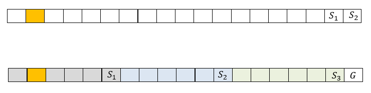
Fig. 1. An example of the display of a stripe RAID6 and stripe LRC

Local checksums are calculated as XOR data blocks on which they depend. There can be several global checksums, they are calculated as RS checksums. In this case, to restore the block number 2, you need to read 6 blocks. This is 3 times less than in the previous case, but it will take more space to store checksums here. It should be noted that in the event of a failure of 2 disks of the same group, the LRC is easily converted to the classic RS by adding (XOR) all 3 local checksums.

Using LRC can perfectly solve the problem of the number of readings needed to restore a single disk. However, if all stripes are placed on disks or cluster nodes in the same way and the sequence of blocks is not changed, it turns out that when changing data in any block of the local group, the local checksum of this group and the global checksum will always be recalculated. Thus, components with checksums will be subject to heavy loads and wear. Therefore, the performance of such an array will be lower. Classically, such a problem in RAID is solved by cyclically shifting stripes on disks, see fig. 2

So that when restoring data, the recovery rate is not limited to the write speed on one component of the storage system, so-called Empty Block (E) can be added to each strip, as is done in RAID-5E and RAID-6E. Thus, the recovered data in each stripe is recorded on its empty block, and therefore on a separate disk. The presence of an empty block in the stripe is optional. In our further reasoning, we will consider stripes with such a block to complete the picture.

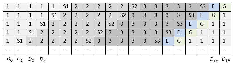
Fig. 2. Location of stripe blocks with shift

Thus, with the use of cyclic shift and the presence of an empty block, the arrangement of stripes on the disks will look like in fig. 2

The use of LRC also imposes a slight limit on the number of disks on which the strip can be located. So, if the number of local groups is

k

$k$ , the size of one local group is equal

l

$l$ , the number of global checksums equals

g

$g$ and there is an empty block, then the total size of the stripe will be equal to

k l + g + 1

$kl + g + 1$ . If the number of disks differs from the stripe length, then two options are possible:

Create local groups of different sizes. In this case, some local checksums will be updated more often when the stripe data changes, which may lead to a slower recording.
Do not place each stripe on all discs, and where one stripe ends, immediately start the second one, see fig. 3. This approach leads to the fact that all local groups can be of the same size, and the cyclic shift is introduced automatically according to the location of the stripes. If the stripe length coincides with the number of disks, then for each stripe a cyclic shift is performed, as is done for RAID-6.

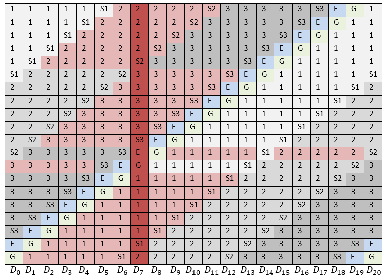
Fig. 3. Blocks needed to repair a single failed disk

In fig. 3 considered the case of failure of one disk -

D_{7}

$D_7$ . Pink color indicates all the blocks that must be read in order to restore it.

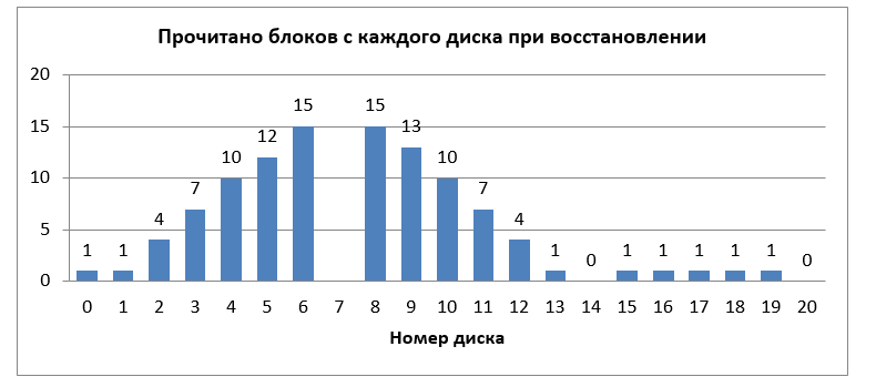
Fig. 4. The number of blocks read from each disk to recover one failed disk.

Total required to read 105 blocks. If RAID-6 were used instead of LRC, then 340 read blocks would be necessary. To understand whether such an arrangement of blocks is optimal, we calculate the number of blocks read from each disk, see fig. four.

You may notice that the disks, which are located closer to the failed one, will be much more loaded compared to the others. Thus, when recovering data in the event of a failure, these most loaded disks will become a bottleneck. However, the location of the LRC-stripe blocks, when the blocks of the first local group come first, then the second, then the third, is not a strict limitation. Thus, our task is to determine the location of the blocks in which the load on all the disks in case of failure would be minimal and uniform.

Randomized algorithms for large disks

Leaving aside the various ways to solve a similar problem for RAID-6, consider a possible scenario in the case of LRC:

For each LRC-stripe, we take the classic arrangement of the blocks (similar to Fig. 1). Use the number of the selected stripe as the initial value (seed) for the random number generator. For all stripes the same random number generator is used, but with different seed.
Using the initiated random number generator and the initial arrangement of the blocks, we obtain a random arrangement of the blocks in the current stripe. In our case, the Fisher – Yates shuffle algorithm was applied.
This procedure is performed for each stripe.

With this approach, each stripe will have some random structure, which is uniquely determined by its number. Since this task does not require the cryptographic strength of a random number generator, we can use a fairly simple and fast version of it. Thus, it is possible to estimate the expectation of the average load of each disk in case of failure.

We introduce the notation:

V

$V$ - the volume of each disk in the array,

s

$s$ - size of one stripe block,

N

$N$ - the length of one stripe,

n

$n$ - the number of disks

l

$l$ - the size of the local group.

k

$k$ - the number of local groups

g

$g$ - the number of global checksums. Then the expectation of the average load of each disk will be calculated as follows:

M (D_{i}) = f r a c V k (l - 1) (l + g) s (n - 1)

$M (D_i) = \ frac {Vk (l-1) (l + g)} {s (n-1)}$

Having such an estimate and knowing the speed of reading blocks from a disk, one can make an approximate estimate of the recovery time of one failed disk.

Performance testing

To test performance, we created a RAID of 22 disks with different layouts. A RAID device was created using a device-mapper modification that changed the addressing of a block of data according to a specific algorithm.

Data was written to the RAID for which checksums were calculated for later recovery. A failed disk was selected. Data recovery was performed either to the corresponding empty blocks or to the hot spare disk.

We compared the following schemes:

RAID-6 - Classic RAID-6 with two checksums; data recovery on hot spare disk;
RAID-6E - RAID6 with an empty block at the end of the stripe; data recovery on empty blocks of the respective stripes;
Classic LRC + E - LRC-scheme in which local groups go sequentially and end with a checksum (see Fig. 3); restore to empty block;
LRC rand - to generate each LRC stripe, its number is used as the core of the random number generator, data recovery to an empty block.

22 disks with the following characteristics were used for testing:

MANUFACTURER: IBM
PART NUMBER: ST973452SS-IBM
CAPACITY: 73GB
INTERFACE: SAS
SPEED: 15K RPM
SIZE FORM FACTOR: 2.5IN

When testing performance, the size of stripe blocks plays an important role. Reading data from disks during data recovery is performed at increasing addresses (sequentially), but due to declustering in random layouts, some blocks are skipped. This means that when working with small blocks, the positioning of the magnetic disk head will be done very often, which will have a detrimental effect on performance.

Since the specific values of the data recovery rate may depend on the hard drive model, manufacturer, RPM, etc., we presented the results in relative terms. Figure 5. shows the performance gains in the considered circuits (RAID6 with an empty block, Classic LRC, LRC rand) in comparison with classic RAID-6.

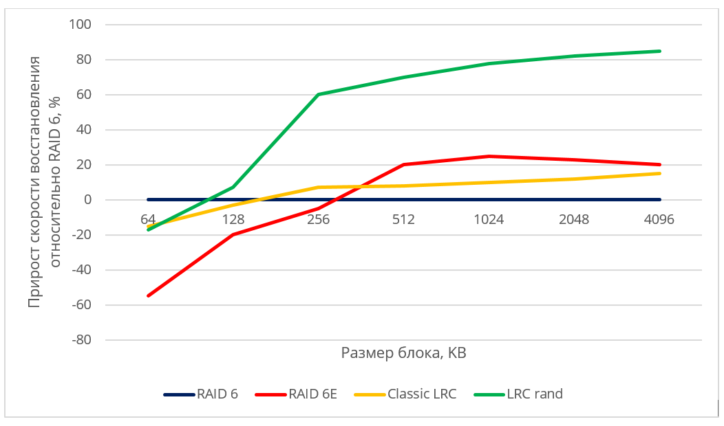
Fig. 5. Relative performance of various placement algorithms

When restoring data to a hot spare disk, the recovery speed was limited by the speed of writing to the disk for all schemes using hot spare. It can be seen that the randomized LRC scheme gives a fairly high increase in the recovery rate compared to the non-optimal scheme and RAID-6.

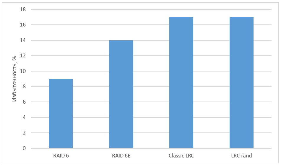
Fig. 6. Redundancy of various algorithms

Conclusion

We gave possible options for the location of the blocks, as well as tested various schemes and saw a noticeable increase in the recovery rate. Due to the high scalability of LRC codes, this approach can also be used when building arrays from a large number of disks, by increasing the number of local groups. Increased reliability can be achieved by increasing the number of global checksums.

The noise-tolerant coding using LRC contributes to a significant reduction in storage redundancy compared to replication. Coding schemes that differ from Reed-Solomon codes are most often studied in practice in the context of LRC. Xorbas - the implementation of LRC in HDFS - demanded an increase in redundancy of 14% compared with RS-coding. The recovery rate at the same time increased by 25-45%. The number of reads and transfers over the network has also been significantly reduced. For further study of the optimal LRC, we recommend to refer to the work “A Family of Optimal Locally Recoverable Codes” (Itzhak Tamo, Alexander Barg).

Used sources:

Hafner, JL, WEAVER Codes: Highly Fault Tolerant Erasure Codes for Storage Systems, FAST-2005: 4th Usenix Conference on File and Storage Technologies
Khan, O., Burns, R., Plank, JS, Pierce, W., Huang, C. Erasure Rethinking Cossacks: FTA-2012: 10th Usenix Conference on File and Storage Technologies
Huang, C., Simitci, H., Xu, Y., Ogus, A., Calder, B., Gopalan, P., Li, J., Yekhanin, S., Erasure Coding in Windows Azure Storage, USENIX Annual Technical Conference
M. Sathiamoorthy, M. Asteris, D. Papailiopoulos, AG Dimakis, R. Vadali, S. Chen, and D. Borthakur. XORing Elephants: Novel Erasure Codes for Big Data. In Proceedings of the VLDB Endowment, volume 6, pages 325–336. VLDB Endowment, 2013.
Itzhak Tamo, Alexander Barg. A Family of Optimal Locally Recoverable Codes. arXiv preprint arXiv: 1311.3284, 2013.

Source: https://habr.com/ru/post/330530/

All Articles