Addition to the analysis of algorithms

This article continues the introductory article on the asymptotic analysis of the complexity of algorithms on Habré. Here you will learn about smoothed analysis and features of the analysis of algorithms in external memory. Inquisitive waiting for links to additional material, and in the end I eat a polynomial.

What you need to know before starting?

On duty, I interviewed students for internship programs and training courses. None of those students knew a clear definition of “O” —big. Therefore, I highly advise you to turn to mathematical literature for such a definition. Basic information in a popular form you will find in the series of articles "Introduction to the analysis of the complexity of algorithms"

Smoothed analysis

Most likely, you hear this phrase for the first time. This is not surprising, since Smoothed analysis appeared by the standards of mathematics recently: in 2001. Of course, this implies that the idea does not lie on the surface. I will assume that you already know the worst case analysis, the average analysis, as well as the relatively useless analysis of the best case: and that three obvious options. So smoothed analysis is the fourth option.

Before explaining why it was needed, it is easier to first clarify why the previous three were invented. I know three key situations in which asymptotic analysis helps:
')
- During the defense of a thesis on mathematics.
- When you need to understand why one algorithm is faster than another or consumes less memory.
- When it is necessary to predict the growth of the operation time or the used memory of the algorithm, depending on the growth of the input size.

The last point is fair with reservations. Due to the fact that real iron is complicated , a theoretical assessment of the nature of growth will work as a bottom estimate for what you will see in the experiment. I deliberately omit the decoding of the word "difficult", because It will take a lot of time. Therefore, I hope that the reader will nod understandingly and will not interrogate me.

For our purposes, it is important to clarify that the asymptotic estimate does not say which algorithm is faster, and certainly does not say anything about a specific implementation. Asymptotics predicts the overall appearance of the growth function, but not absolute values. Algorithms for rapid multiplication are a textbook example of such a situation: the Karatsuba method overtakes the naive only after reaching a length of "several dozen characters", and the Schönhage-Strassen method overtakes the Karatsuba method with a length of "from 10,000 to 40,000 decimal places." It is impossible to draw such conclusions without experiment, if we only look at the asymptotics.

On the other hand, having on hand the results of the experiment it is impossible to conclude that this trend will always continue or that we are not lucky with the input data. In this situation, the asymptotic analysis helps, which helps to prove why the algorithm for sorting Hoare is faster than a bubble. In other words, both experimental data and theoretical results are necessary for complete understanding and peace of mind.

This explains the presence of one asymptotic estimate, but why should the others? It's simple. Suppose the two algorithms have an asymptotic worst case estimate of the same, and the experimental results indicate clear advantages of one over the other. In such a situation, it is necessary to analyze the average case in search of a difference that will explain everything. This is what happens when comparing the sorting of Hoar and the bubble, in which the asymptotically identical worst case but different average.

Smoothed score is midway between middle and worst case. It is written as:

$$

$$_ {smooth} (n, \ sigma) = \ max \ limits_ {x} \ {M_ {r \ in X_ {n}} [\ tau (x + \ sigma || x || r)] \}$$

where $$$\ sigma$some small constant $$$X_n$plenty of possible size input $$$n$, $$$\ tau$a function that returns the time (or memory) that the algorithm spends on processing specific data, $$$M$- the expectation, and the brackets are different for convenience.

In simple terms, smooth estimation means that there is not a sufficiently large continuous piece of data on which the algorithm will run on average slower than $$$C_ {smooth}$. Thus the smoothed score is stronger than average, but weaker than the worst. Obviously varying $$$\ sigma$you can shift it from average to maximum.

Since the definition is not trivial, I drew a picture to understand:

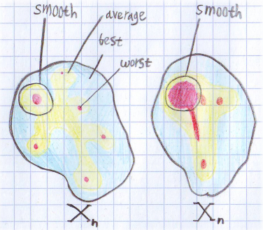Here we draw the distribution of time over the set of input data for some n. Red areas - the worst case, yellow - medium, and blue - the best. For the left set, the average and smoothed score will be about the same. But for the right smoothed score will be closer to the worst case. For both sets, the smoothed score more accurately describes the behavior of the algorithm. If we imagine that both figures correspond to the same task, but to different algorithms, an interesting situation is obtained. They rate the best, worst and average cases the same. But in practice, the left-handed algorithm will feel better because on the right is much easier to arrange an algorithmic attack.

Read more about this in the article "Smoothed Analysis of Algorithms" . It uses this approach to analyze the simplex method. The links can be found and other articles.

Analysis of algorithms in external memory

Before talking about algorithms in external memory, it is worth emphasizing one thing that bypasses. The theoretical estimates, which were discussed, are formally derived not wherever, but in a model called “RAM machine”. This is a model in which access to an arbitrary place of memory occurs in one elementary operation. Thus, you equate computational and memory operations, which simplifies the analysis.

External memory is a disk, network, or other slow device. To analyze the algorithms operating with them, use a different execution model in external memory. If to simplify, then in this model the computer has $$$M$machine words of internal memory, all operations with which cost nothing, just as no computation operations cost anything on the CPU, and there is still external memory with which it is possible to work only with whole blocks of size $$$B$words and each such operation is considered elementary. And $$$M$much bigger $$$B$. In this model, they talk about IO complexity of the algorithm.

Thus, even if you solve an NP-complete problem in memory on each block, this will not affect the IO-complexity of the algorithm. But in such a wording, this is not a big problem, since the block has a fixed length and we simply say that this is our elementary operation. However, the model will not be applicable to the algorithm dramatically reducing the number of operations on the CPU at the cost of increasing disk operations, so in the end it will be beneficial. But even in this case, it is necessary that this exchange be non-trivial. Moreover, the exchange in the opposite direction fits into the model, so adding compression does not cause difficulties. A replacement of the slow compression algorithm for a faster, refers to the trivial exchange.

The second difference from the RAM model is the format of operations. It is possible to operate only with large continuous blocks. This reflects the work with the disks in practice. Which in turn is due to the fact that the discs have a gap between the speed of consecutive operations compared with the internal memory is smaller than the similar gap between an operation with an arbitrary cell. Thus, it is advantageous to level the positioning time. In the model, we simply say that we succeeded and there is no positioning time, but there are continuous blocks of length $$$B$sufficient that the model is correct.

When analyzing in this model, be careful with rounding, as reading one machine word and $$$B$machine words takes the same time. Generally reading $$$N$consecutive words takes $$$\ lceil N / B \ rceil$operations, and with small $$$N$the rounding contribution will be significant, especially if this value is then multiplied by something.

Because of the peculiarities of the model, problems begin to be solved as if faster, since computational operations cost nothing. For example, merge sorting is performed for $$$O (\ frac {Nlog_ {M / B} (N / B)} {B})$that much faster than it could be. But do not be fooled, with fixed $$$M$and $$$B$, all this gives only a multiplicative constant, which is easily eaten by the disk.

SSD and cache

There are two topics that can not be circumvented. Let's start with the cache. The logic is approximately the following: in general, the cache and RAM ratios are similar to the memory and disk ratios. But there is one caveat: RAM has no lag for random access. Despite the fact that reading from L1 cache is about 200 times faster than reading from memory, it’s still the basis of the model in the search lag. There is an alternative formulation of the question: to create an algorithm so as to minimize the number of cache misses, but this is a topic for another conversation.

SSD is only 4 times slower than memory for sequential reading, but 1,500 times slower for random reading. That is why the model as a whole is fair for him, since you will still want to level the search lag.

Thus, this model, though simple, remains correct in a large number of cases. In more detail about algorithms in external memory with the examples of the analysis I suggest to get acquainted with the course of Maxim Babenko from 5 lectures .

Bonus

Finally, I will talk about the interesting notation used in the analysis of NP-complete problems. I myself learned about such a designation in the lectures by Alexander Kulikov “Algorithms for NP-hard problems” .

Informally, the symbol “O” -big eats everything except the older member, and at the older member eats the multiplicative constant. It turns out that there is a symbol $$$O ^ {\ ast}$which eats up not just a multiplicative constant, but a whole polynomial. Those. $$$O (n ^ {100}) = O ^ {\ ast} (1)$and $$$O (n ^ {100} 2 ^ n) = O ^ {\ ast} (2 ^ n)$. So if you feel sad because your program is slow, you can console yourself with the thought that its IO complexity is algorithmically $$$O ^ * (1)$.