A review of research in the field of deep learning: natural language processing

This is the third article in the “Deep Learning Research Review” series of UCLA student Adit Deshpande. Every two weeks Adit publishes a review and interpretation of research in a specific area of ​​in-depth training. This time, he focused on applying deep learning to natural language processing.

Introduction to natural language processing

Introduction

Natural language processing (NLP) is the creation of systems that process or “understand” the language in order to accomplish certain tasks. These tasks may include:

• Question Answering (what Siri, Alexa and Cortana do)
• Analysis of the emotional coloration of statements (Sentiment Analysis) (determination of whether the statement has a positive or negative connotation)
• Finding the text corresponding to the image (Image to Text Mappings) (generating a signature for the input image)
• Machine Translation (text paragraph translation from one language to another)
• Speech Recognition
• Part of Speech Tagging (definition of parts of speech in a sentence and their annotation)
• Extract Entities (Name Entity Recognition)

The traditional approach to NLP suggested a deep knowledge of the subject area - linguistics. The understanding of such terms as phonemes and morphemes was obligatory, since there are whole disciplines of linguistics devoted to their study. Let's see how traditional NLP would recognize the following word:

Suppose our goal is to collect some information about this word (determine its emotional coloring, find its meaning, etc.). Using our knowledge of the language, we can break this word into three parts.

')
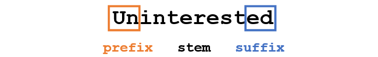
We understand that the prefix (prefix) un- means negation, and we know that -ed can mean the time to which a given word belongs (in this case, the past tense). Recognizing the meaning of the single-parent word interest, we can easily conclude about the meaning and emotional coloring of the whole word. It seems to be simple. However, if you take into account the diversity of prefixes and suffixes of the English language, you will need a very skilled linguist to understand all the possible combinations and their meanings.


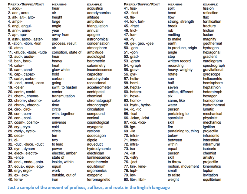
An example showing the number of suffix prefixes and roots in English

How to use deep learning

At the heart of deep learning is the teaching of ideas. For example, convolutional neural networks (CNN) include a combination of different filters designed to categorize objects into categories. Here we will try to apply a similar approach by creating representations of words in large data sets.

Article structure

This article is organized so that we can go through the basic elements from which you can build deep networks for NLP, and then proceed to discuss some of the applications that are related to recent scientific work. It's okay if you don’t know exactly why, for example, we use RNN, or LSTM is useful, but hopefully, having studied these works, you will understand why deep learning is so important for NLP.

Word vectors

Since deep learning cannot live without mathematics, let us represent each word as a d-dimensional vector. Take d = 6.

Now we will think how to fill the values. We want the vector to be filled in such a way that it somehow represents the word and its context, meaning, or semantics. One of the ways is to build a co-occurrence matrix. Consider the following sentence:

We want to get a vector representation for each word.


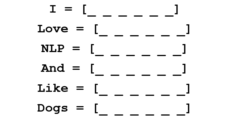
The co-occurrence matrix contains the number of times each word has been encountered in the corpus (training set) after each other word of this corpus.



The rows of this matrix can serve as vector representations of our words.

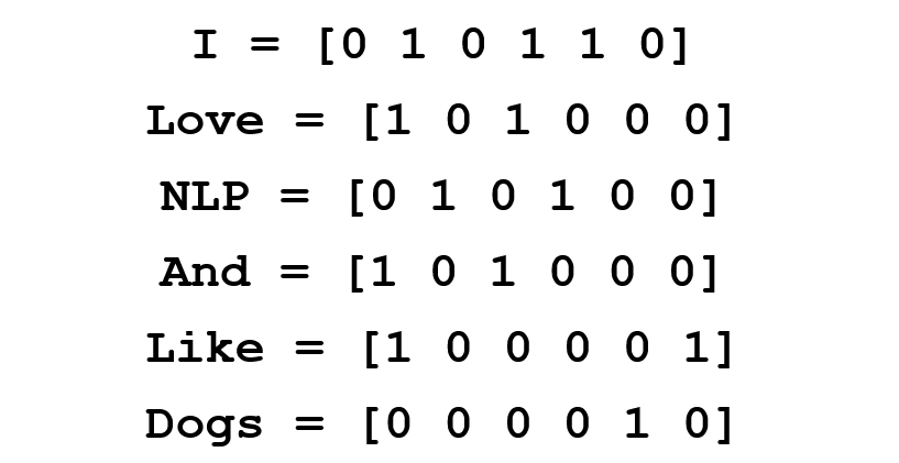
Please note that even from this simple matrix we can gather some rather important information. For example, note that the vectors of the words “love” and “like” contain units in the cells responsible for their proximity to nouns (“NLP” and “dogs”). They also have “1” where they are next to “I”, indicating that this word is most likely a verb. You can imagine how much easier it is to identify similar similarities when a data set is more than one sentence: in this case, the vectors of verbs such as “love”, “like” and other synonyms will be similar, since these words will be used in similar contexts.

Good for a start, but here we note that the dimension of the vector of each word will increase linearly depending on the size of the body. In the case of a million words (which is a little for standard NLP tasks), we would get a million-million-by-one matrix, which, moreover, would be very sparse (with a lot of zeros). This is definitely not the best option in terms of data storage efficiency. In the issue of finding the optimal vector representation of words, several serious moves were made. The most famous of them is Word2Vec.

Word2vec

The main goal of all methods for initializing a word vector is to store as much information as possible in this vector, while maintaining a reasonable dimension (ideally, from 25 to 1000). At the heart of Word2Vec is the idea of ​​learning how to predict the surrounding words for each word. Consider the sentence from the previous example: “I love NLP and I like dogs”. Now we are only interested in the first three words. Let the size of our window be three.

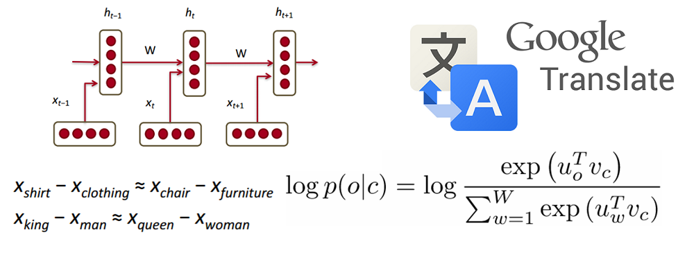
Now we want to take the central word “love” and predict the words going before and after it. How do we do this? Of course, by maximizing and optimizing the function! Formally, our function tries to maximize the logarithmic probability of each word context for the current central word.

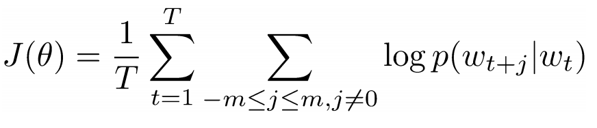
We study the above formula in more detail. It follows from this that we add the logarithmic probability of joint occurrence of both “I” and “love”, and “NLP” and “love” (in both cases, “love” is the central word). The variable T denotes the number of training offers. Consider the logarithmic probability closer.

$$$V_c$- vector representation of the central word. Each word has two vector representations: $$$U_o$and $$$U_w$, one for the case when the word occupies a central position, the other for the case when this word is “external”. Vectors are trained by stochastic gradient descent. This is definitely one of the most difficult to understand equations, so if you still have a hard time imagining what is happening, you can find additional information here and here .

To summarize in one sentence : Word2Vec searches for vector representations of various words, maximizing the logarithmic probability of the occurrence of context words for a given central word and transforming vectors using the method of stochastic gradient descent.

(Optional: further, the authors of the work talk in detail about how using negative sampling and subsampling to get more accurate word vectors).

Perhaps the most interesting contribution of Word2Vec to the development of NLP was the emergence of linear relationships between different word vectors. After learning, vectors reflect various grammatical and semantic concepts.

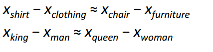
It's amazing how such a simple objective function and simple optimization technique could reveal these linear relationships.

Bonus : another cool method to initialize word vectors is GloVe (Global Vector for Word Representation) (combines the ideas of the co-occurrence matrix with Word2Vec).

Recurrent Neural Networks (Recurrent Neural Networks, RNN)

Now let's see how the recurrent neural network will work with our vectors. RNN is a magic wand for most modern natural language processing tasks. The main advantage of RNN is that they can efficiently use data from previous steps. This is what a small piece of RNN looks like:

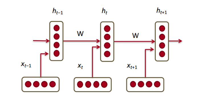
Below are word vectors ( $$$x_t, x_ {t-1}, x_ {t + 1}$). Each vector at each step has a hidden state vector (hidden state vector) ( $$$h_t, h_ {t-1}, h_ {t + 1}$). We will call this pair a module.

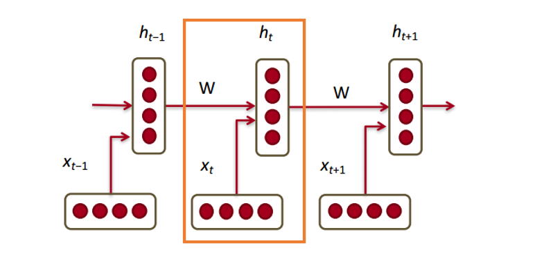
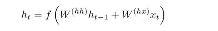
The hidden state in each RNN module is a function of the word vector and the hidden state vector from the last step.

If we take a closer look at superscripts, we will see that there is a weights matrix $$$W ^ {hx}$, which we multiply by the input value, and there is a recurrent matrix of weights $$$W ^ {hh}$which is multiplied by the latent state vector from the previous step. Keep in mind that these recurrent weights matrices are the same at each step. This is the key point of the RNN . If you think carefully, then this approach is significantly different from, say, traditional two-layer neural networks. In this case, we usually choose a separate matrix W for each layer: $$$W_1$and $$$W_2$. Here, the recurrent weights matrix is ​​the same for the entire network.

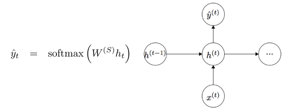
To obtain the output values ​​of each module (Yhat) is another matrix of weights - $$$W ^ s$multiplied by h.


Now let's look from the side and see what the benefits of RNN are. The most obvious difference between the RNN and the traditional neural network is that the RNN accepts input data sequences (in our case, words). In this way, they differ, for example, from typical CNN, to which the whole image is fed to the input. For RNN, however, the input data can be either a short sentence or a five-paragraph essay. In addition, the order in which data is supplied can influence how the weight matrices and the vectors of hidden states change in the learning process. By the end of the training, information from past steps should accumulate in the vectors of hidden states.

Managed recurrent neurons (Gated recurrent units, GRU)

Now let's get acquainted with the concept of a controlled recurrent neuron, which is used to calculate the vectors of hidden states in RNN. This approach allows you to save information about more remote dependencies. Let's speculate why distant dependencies for ordinary RNNs can be a problem. At the time of the back propagation of the error (backpropagation) method, the error will move along the RNN from the last step to the earliest. With a sufficiently small initial gradient (say, less than 0.25) to the third or fourth module, the gradient will almost disappear (since, according to the rule of the derivative of a complex function, the gradients multiply), and then the hidden states of the very first steps will not be updated.

In normal RNN, the vector of hidden states is calculated by the following formula:

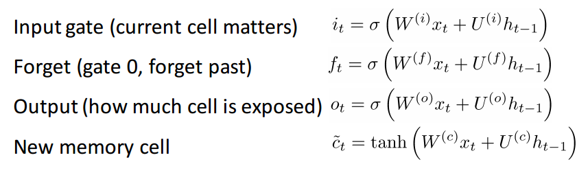
The GRU method allows us to calculate h (t) differently. The calculations are divided into three blocks: an update gate filter, a reset gate filter, and a new memory container. Filter filters are functions of the input vector representation of the word and the hidden state in the previous step.

The main difference is that each filter uses its own weight. This is indicated by different superscripts. Update filter uses $$$W ^ z$and $$$U ^ z$and the state reset filter is $$$W ^ r$and $$$U ^ r$.
Now let's calculate the memory container:

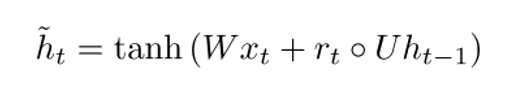
(an empty circle here refers to the work of Hadamard ).

Now, if you look at the formula, you can see that if the factor of the reset filter is close to zero, then the whole product will also approach zero, and thus, the information from the previous step $$$h_ {t-1}$will not be counted. In this case, the neuron is just a function of the new word vector. $$$x_ {t-1}$.

The final formula h (t) can be written as

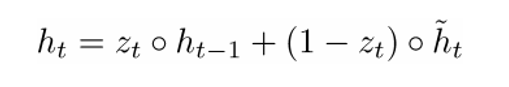
$$$h_t$- a function of all three components: an update filter, a state reset filter, and a memory container. You can better understand this by visualizing what happens to a formula when $$$z_t$nearing 1 and when $$$z_t$close to 0. In the first case, the hidden state vector $$$h_t$largely depends on the previous hidden state, and the current memory container is not taken into account, since (1 - $$$z_t$) tends to 0. When $$$z_t$nearing 1, the new vector of the hidden state $$$h_t$, on the contrary, depends mainly on the memory container, and the previous hidden state is not taken into account. So, our three components can be intuitively described as follows:

• Update filter
  
  • If a $$$z_t$~ 1, then $$$h_t$does not take into account the current vector of the word and simply copies the previous hidden state.
  • If a $$$z_t$~ 0, then $$$h_t$does not take into account the previous hidden state and depends only on the memory container.
  • This filter allows the model to control how much information from the previous hidden state should affect the current hidden state.
• State reset filter
  
  • If a $$$r_t$~ 1, the memory container stores information from the previous hidden state.
  • If a $$$r_t$~ 0, the memory container does not take into account the previous hidden state.
  • This filter allows you to discard some of the information, if in the future it will not interest us.
• Memory Container: Depends on the reset filter.

Let us give an example illustrating the work of GRU. Suppose we have the following several sentences:

and the question: “What is the sum of two numbers?” Since the sentence in the middle does not affect the answer, the reset and update filters will allow the model to “forget” this sentence and understand that only certain information can change the hidden state (in this case, numbers) .

Neurons with long short term memory (LSTM)

If you are done with GRU, then LSTM will not be difficult for you. LSTM also consists of a sequence of filters.

LSTM definitely takes in more information. Since it can be considered an extension of GRU, I will not analyze it in detail, but to get a detailed description of each filter and each step of the calculations, you can refer to the beautifully written blog post by Chris Olah. At the moment, this is the most popular LSTM tutorial, and will definitely help those of you who are looking for a clear and intuitive explanation of how this method works.

Comparison of LSTM and GRU

First, consider the common features. Both of these methods are designed to preserve distant dependencies in sequences of words. Distant dependencies mean situations where two words or phrases can occur at different time steps, but the relationship between them is important for achieving the ultimate goal. LSTM and GRUs track these relationships using filters that can save or discard information from the sequence being processed.

The difference between the two methods is in the number of filters (GRU - 2, LSTM - 3). This affects the amount of nonlinearity that comes from the input data and ultimately affects the calculation process. In addition, there is no memory in the GRU. $$$c_t$as in lstm.

Before going into articles

I would like to make a small note. If other models of deep learning, useful in NLP. In practice, recursive and convolutional neural networks are sometimes used, although they are not as common as the RNNs that underlie most NLP deep learning systems.

Now that we have begun to understand well the recurrent neural networks with reference to NLP, let's take a look at some of the work in this area. Since NLP includes several different areas of tasks (from machine translation to forming answers to questions), we could consider quite a lot of work, but I chose the three that I found particularly informative. In 2016, there was a number of significant advances in the field of NLP, but we will start with one work in 2015.

Neural networks with memory (Memory Networks)

Introduction

The first work that we will discuss has had a great influence on the development of the field of forming answers to questions. In this publication, authorship by Jason Weston, Sumit Chopra and Antoine Bordes first described the class of models called “memory network”.

The intuitive idea is this: in order to accurately answer a question relating to a piece of text, you must somehow store the source information provided to us. If I asked you: “What does the abbreviation RNN mean?”, You could answer me, because the information that you learned while reading the first part of the article was stored somewhere in your memory. You only need a few seconds to find this information and voice it. I have no idea how it works in the brain, but the idea that space is needed to store this information remains unchanged.

The memory network described in this paper is unique because it has an associative memory to which it can write and from which it can read. It is interesting to note that neither CNN, nor Q-Network (for reinforcement learning), nor traditional neural networks use such memory, this is partly due to the fact that the task of forming answers to questions relies heavily on the ability to model or track remote dependencies, for example, keep track of the heroes of the story, or memorize the sequence of events. It would be possible to use RNN or LSTM, but usually they are not able to remember input data from the past (which is critical for the tasks of forming answers to questions).

Network architecture

Now let's see how this network handles the source code. Like most machine learning algorithms, the first step is to convert the input data into a feature space representation. This may include the use of vector representations of words, morphological markup, syntactic analysis, etc., at the discretion of the programmer.

The next step is to take a representation in the feature space I (x) and read into memory the new portion of the input data x.

Memory m can be considered as the similarity of an array made up of individual blocks of memory. $$$m_i$. Every such block $$$m_i$may be a function of the entire memory m, the representation in the feature space I (x) and / or itself. The G function can simply store the entire representation I (x) in the memory block mi. Function G can be modified to update the memory of the past based on new input data. The third and fourth steps include reading from memory, taking into account the question, to find a representation of the signs o, and decoding it, to get the final answer r.

RNN can serve as a function of R, which transforms the presentation of signs into human-readable and accurate answers to questions.

Now let's take a closer look at step 3. We want the function O to return a representation in the feature space that best matches the possible answer to the asked question x. , .

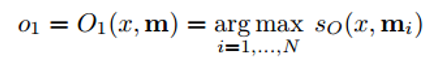
(argmax) , , ( , ). ( ) ( ). , , . RNN, LSTM , .

, , , . , :



, , , :

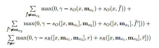
• End to End Memory Networks
• Dynamic Memory Networks
• Dynamic Coattention Networks ( 2016 Stanford's Question Answering)

Tree-LSTM

Introduction

– , (). “ ”. LSTM. (Kai Sheng Tai), (Richard Socher) (Christopher Manning) LSTM- .

, . , , , . , LSTM- , .

Tree-LSTM LSTM , – . Tree-LSTM – .

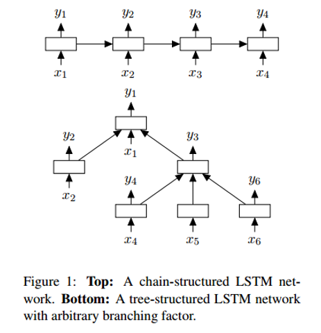
– – , , . . , LSTM.

Tree-LSTM . , -. , (, “” “”) . .

(Neural Machine Translation, NMT)

Introduction

, , . – Google (Jeff Dean), (Greg Corrado), (Orial Vinyals) – , Google Translate. 60% , Google.

. . , . , ( NMT) , .

LSTM, . : RNN, RNN “” (attention module). , , , ( ).

, . , , .

Conclusion

, . , , , , (, ).

Oh, and come to work with us? :)

wunderfund.io is a young foundation that deals with high-frequency algorithmic trading . High-frequency trading is a continuous competition of the best programmers and mathematicians of the whole world. By joining us, you will become part of this fascinating fight.

We offer interesting and challenging data analysis and low latency tasks for enthusiastic researchers and programmers. Flexible schedule and no bureaucracy, decisions are quickly made and implemented.

Join our team: wunderfund.io