Load optimization in the “Remains in warehouses” task using partitioning in SQL Server
This article provides a Transact SQL optimization solution for calculating stock balances. Applied: partitioning of tables and materialized views.
The task needs to be solved on SQL Server 2014 Enterprise Edition (x64). The company has many warehouses. In each warehouse every day for several thousand shipments and acceptance of products. There is a table of movements of goods in the stock receipt / consumption. It is necessary to implement:
Calculation of the balance on the selected date and time (up to an hour) for all / any warehouses for each product. For analytics, it is necessary to create an object (function, table, view) with the help of which, for the selected date range, output the source table data for all warehouses and products and the additional calculation column - the balance in the position warehouse.
')
These calculations are supposed to be performed on a schedule with different date ranges and should work at an acceptable time. Those. if it is necessary to display a table with residuals for the last hour or day, the execution time should be as fast as possible, as well as if it is necessary to output the same data for the last 3 years, for subsequent loading into the analytical database.
Technical details. The table itself:
Create a filled table. In order to test and watch the results with me, I suggest creating and filling in the dbo.Turnover table with a script:
I had this script on a PC with an SSD disk running for about 22 minutes, and the size of the table took about 8GB on the hard disk. You can reduce the number of years, and the number of warehouses, in order to reduce the time for creating and filling the table. But I recommend to leave some good volume for evaluating query plans, at least 1-2 gigabytes.
Group data up to an hour
Further, we need to group the amounts by products in stock for the studied period of time, in our formulation of the task it is one hour (you can up to a minute, up to 15 minutes, a day. But it is obvious that milliseconds hardly anyone will need reporting). For comparisons in the session (window) where we execute our requests, we execute the command - set statistics time on ;. Next, we execute the queries themselves and look at the query plans:
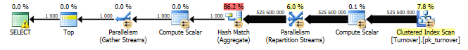
If we make the resulting query with a balance, which is considered to be a cumulative total of our quantity, then the query and the query plan will be as follows:
Group optimization
It's pretty simple here. The query itself without a cumulative total can be optimized with a materialized view (index view). To build a materialized view, what is summed should not be NULL, we sum the sum (Operation * Quantity), or make each field NOT NULL or add isnull / coalesce to the expression. I propose to create a materialized view.
And build a clustered index on it. In the index, we specify the order of the fields in the same way as in the grouping (for grouping, so much order is not important, it is important that all fields of the grouping be in the index) and progressively (here the order is important - first what's in partition by, then what's in order by):
Now, after building the cluster index, we can re-execute queries by changing the aggregation of the amount as in the view:
Query plans have become:
 Cost 0.008
 Cost 0.01
So, we see that with an indexed view, the query scans not the table grouping the data, but the cluster index, in which everything is already grouped. And accordingly, the execution time was reduced from 321797 milliseconds to 116 ms, i.e. 2774 times.
This would allow us to finish our optimization, if not for the fact that we often need not the entire table (view), but its part for the selected range.
Intermediate Balances
As a result, we need fast execution of the following query:
Cost of the plan = 3103. But imagine what would have happened if it were not for the materialized view, but for the table itself.
Data output materialized view and balance for each product in stock at a date with a time rounded up to an hour. In order to calculate the balance, it is necessary from the very beginning (from zero balance) to sum all the quantities up to the specified last date (@finish), and then cut the data later than the start parameter in the summarized result set.
Here, obviously, intermediate calculated balances will help. For example, on the 1st day of each month or on every Sunday. Having such balance sheets, the task comes down to the fact that it will be necessary to sum up previously calculated balance sheets and calculate the balance not from the beginning, but from the last calculated date. For experiments and comparisons, we will build an additional non-cluster index by date:
In general, this query, having even an index by date completely covering all the fields affected by the query, will select our clustered index and scan. And not search by date, followed by sorting. I propose to perform the following 2 requests and compare what we have obtained, then we will analyze what is still better:
From the time it is clear that the index by date runs much faster. But query plans in comparison are as follows:
The cost of the 1st request with the automatically selected cluster index = 2752, but the cost with the index by the request date = 3119.
However, here we need two tasks from the index: sorting and sampling the range. One index from available to us not to solve this task. In this example, the data range is just 1 day, but if there is a longer period, but not all, for example, 2 months, then an unequivocal index search will not be effective due to the cost of sorting.
Here, from the visible optimal solutions, I see:
In the project as a result I made the 3rd option. Partitioning a clustered index of a materialized view. And if the sample goes for a period of one month, then in fact the optimizer affects only one section, making it scan without sorting. And the cut-off of unused data occurs at the cut-off level of unused sections. Here, if the search from the 10th to the 20th day we do not have an exact search for these dates, but a search for data from the 1st to the last day of the month, further scanning of this range in a sorted index filtered during the scanning by the set dates.
We partition the cluster index of the view. First of all, let's remove all indexes from the view:
And create a function and partitioning scheme:
In fact, data in one section is selected and scanned by a cluster index rather quickly. It should be added here that when the request is parameterized, the unpleasant effect of parameter sniffing occurs, the option (recompile) is treated.
Formulation of the problem
The task needs to be solved on SQL Server 2014 Enterprise Edition (x64). The company has many warehouses. In each warehouse every day for several thousand shipments and acceptance of products. There is a table of movements of goods in the stock receipt / consumption. It is necessary to implement:
Calculation of the balance on the selected date and time (up to an hour) for all / any warehouses for each product. For analytics, it is necessary to create an object (function, table, view) with the help of which, for the selected date range, output the source table data for all warehouses and products and the additional calculation column - the balance in the position warehouse.
')
These calculations are supposed to be performed on a schedule with different date ranges and should work at an acceptable time. Those. if it is necessary to display a table with residuals for the last hour or day, the execution time should be as fast as possible, as well as if it is necessary to output the same data for the last 3 years, for subsequent loading into the analytical database.
Technical details. The table itself:
create table dbo.Turnover ( id int identity primary key, dt datetime not null, ProductID int not null, StorehouseID int not null, Operation smallint not null check (Operation in (-1,1)), -- +1 , -1 Quantity numeric(20,2) not null, Cost money not null ) Dt - Date the time of receipt / debiting to / from the warehouse.
ProductID - Product
StorehouseID - warehouse
Operation - 2 values of arrival or consumption
Quantity - the amount of product in stock. It may be material if the product is not in pieces, but, for example, in kilograms.
Cost - the cost of the product batch.
Research task
Create a filled table. In order to test and watch the results with me, I suggest creating and filling in the dbo.Turnover table with a script:
if object_id('dbo.Turnover','U') is not null drop table dbo.Turnover; go with times as ( select 1 id union all select id+1 from times where id < 10*365*24*60 -- 10 * 365 * 24 * 60 = 10 ) , storehouse as ( select 1 id union all select id+1 from storehouse where id < 100 -- ) select identity(int,1,1) id, dateadd(minute, t.id, convert(datetime,'20060101',120)) dt, 1+abs(convert(int,convert(binary(4),newid()))%1000) ProductID, -- 1000 - s.id StorehouseID, case when abs(convert(int,convert(binary(4),newid()))%3) in (0,1) then 1 else -1 end Operation, -- , 3 2 1 1+abs(convert(int,convert(binary(4),newid()))%100) Quantity into dbo.Turnover from times t cross join storehouse s option(maxrecursion 0); go --- 15 min alter table dbo.Turnover alter column id int not null go alter table dbo.Turnover add constraint pk_turnover primary key (id) with(data_compression=page) go -- 6 min I had this script on a PC with an SSD disk running for about 22 minutes, and the size of the table took about 8GB on the hard disk. You can reduce the number of years, and the number of warehouses, in order to reduce the time for creating and filling the table. But I recommend to leave some good volume for evaluating query plans, at least 1-2 gigabytes.
Group data up to an hour
Further, we need to group the amounts by products in stock for the studied period of time, in our formulation of the task it is one hour (you can up to a minute, up to 15 minutes, a day. But it is obvious that milliseconds hardly anyone will need reporting). For comparisons in the session (window) where we execute our requests, we execute the command - set statistics time on ;. Next, we execute the queries themselves and look at the query plans:
select top(1000) convert(datetime,convert(varchar(13),dt,120)+':00',120) as dt, -- ProductID, StorehouseID, sum(Operation*Quantity) as Quantity from dbo.Turnover group by convert(datetime,convert(varchar(13),dt,120)+':00',120), ProductID, StorehouseID Request price - 12406
(lines processed: 1000)
SQL Server running time:
CPU time = 2096594 ms, elapsed time = 321797 ms.
If we make the resulting query with a balance, which is considered to be a cumulative total of our quantity, then the query and the query plan will be as follows:
select top(1000) convert(datetime,convert(varchar(13),dt,120)+':00',120) as dt, -- ProductID, StorehouseID, sum(Operation*Quantity) as Quantity, sum(sum(Operation*Quantity)) over ( partition by StorehouseID, ProductID order by convert(datetime,convert(varchar(13),dt,120)+':00',120) ) as Balance from dbo.Turnover group by convert(datetime,convert(varchar(13),dt,120)+':00',120), ProductID, StorehouseID Request price - 19329
(lines processed: 1000)
SQL Server running time:
CPU time = 2413155 ms, elapsed time = 344631 ms.
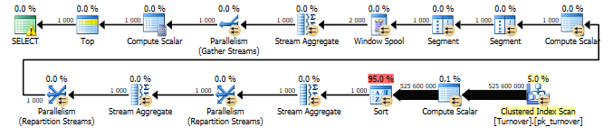
Group optimization
It's pretty simple here. The query itself without a cumulative total can be optimized with a materialized view (index view). To build a materialized view, what is summed should not be NULL, we sum the sum (Operation * Quantity), or make each field NOT NULL or add isnull / coalesce to the expression. I propose to create a materialized view.
create view dbo.TurnoverHour with schemabinding as select convert(datetime,convert(varchar(13),dt,120)+':00',120) as dt, -- ProductID, StorehouseID, sum(isnull(Operation*Quantity,0)) as Quantity, count_big(*) qty from dbo.Turnover group by convert(datetime,convert(varchar(13),dt,120)+':00',120), ProductID, StorehouseID go And build a clustered index on it. In the index, we specify the order of the fields in the same way as in the grouping (for grouping, so much order is not important, it is important that all fields of the grouping be in the index) and progressively (here the order is important - first what's in partition by, then what's in order by):
create unique clustered index uix_TurnoverHour on dbo.TurnoverHour (StorehouseID, ProductID, dt) with (data_compression = page) - 19 minNow, after building the cluster index, we can re-execute queries by changing the aggregation of the amount as in the view:
select top(1000) convert(datetime,convert(varchar(13),dt,120)+':00',120) as dt, -- ProductID, StorehouseID, sum(isnull(Operation*Quantity,0)) as Quantity from dbo.Turnover group by convert(datetime,convert(varchar(13),dt,120)+':00',120), ProductID, StorehouseID select top(1000) convert(datetime,convert(varchar(13),dt,120)+':00',120) as dt, -- ProductID, StorehouseID, sum(isnull(Operation*Quantity,0)) as Quantity, sum(sum(isnull(Operation*Quantity,0))) over ( partition by StorehouseID, ProductID order by convert(datetime,convert(varchar(13),dt,120)+':00',120) ) as Balance from dbo.Turnover group by convert(datetime,convert(varchar(13),dt,120)+':00',120), ProductID, StorehouseID Query plans have become:
Cost 0.008 Cost 0.01SQL Server running time:
CPU time = 31 ms, elapsed time = 116 ms.
(lines processed: 1000)
SQL Server running time:
CPU time = 0 ms, elapsed time = 151 ms.
So, we see that with an indexed view, the query scans not the table grouping the data, but the cluster index, in which everything is already grouped. And accordingly, the execution time was reduced from 321797 milliseconds to 116 ms, i.e. 2774 times.
This would allow us to finish our optimization, if not for the fact that we often need not the entire table (view), but its part for the selected range.
Intermediate Balances
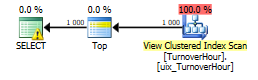
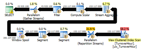
As a result, we need fast execution of the following query:
set dateformat ymd; declare @start datetime = '2015-01-02', @finish datetime = '2015-01-03' select * from ( select dt, StorehouseID, ProductId, Quantity, sum(Quantity) over ( partition by StorehouseID, ProductID order by dt ) as Balance from dbo.TurnoverHour with(noexpand) where dt <= @finish ) as tmp where dt >= @start Cost of the plan = 3103. But imagine what would have happened if it were not for the materialized view, but for the table itself.
Data output materialized view and balance for each product in stock at a date with a time rounded up to an hour. In order to calculate the balance, it is necessary from the very beginning (from zero balance) to sum all the quantities up to the specified last date (@finish), and then cut the data later than the start parameter in the summarized result set.
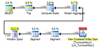
Here, obviously, intermediate calculated balances will help. For example, on the 1st day of each month or on every Sunday. Having such balance sheets, the task comes down to the fact that it will be necessary to sum up previously calculated balance sheets and calculate the balance not from the beginning, but from the last calculated date. For experiments and comparisons, we will build an additional non-cluster index by date:
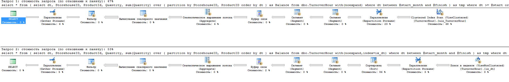
create index ix_dt on dbo.TurnoverHour (dt) include (Quantity) with(data_compression=page); --7 min : set dateformat ymd; declare @start datetime = '2015-01-02', @finish datetime = '2015-01-03' declare @start_month datetime = convert(datetime,convert(varchar(9),@start,120)+'1',120) select * from ( select dt, StorehouseID, ProductId, Quantity, sum(Quantity) over ( partition by StorehouseID, ProductID order by dt ) as Balance from dbo.TurnoverHour with(noexpand) where dt between @start_month and @finish ) as tmp where dt >= @start order by StorehouseID, ProductID, dt In general, this query, having even an index by date completely covering all the fields affected by the query, will select our clustered index and scan. And not search by date, followed by sorting. I propose to perform the following 2 requests and compare what we have obtained, then we will analyze what is still better:
set dateformat ymd; declare @start datetime = '2015-01-02', @finish datetime = '2015-01-03' declare @start_month datetime = convert(datetime,convert(varchar(9),@start,120)+'1',120) select * from ( select dt, StorehouseID, ProductId, Quantity, sum(Quantity) over ( partition by StorehouseID, ProductID order by dt ) as Balance from dbo.TurnoverHour with(noexpand) where dt between @start_month and @finish ) as tmp where dt >= @start order by StorehouseID, ProductID, dt select * from ( select dt, StorehouseID, ProductId, Quantity, sum(Quantity) over ( partition by StorehouseID, ProductID order by dt ) as Balance from dbo.TurnoverHour with(noexpand,index=ix_dt) where dt between @start_month and @finish ) as tmp where dt >= @start order by StorehouseID, ProductID, dt SQL Server running time:
CPU time = 33860 ms, elapsed time = 24247 ms.
(lines processed: 145608)
(lines processed: 1)
SQL Server running time:
CPU time = 6374 ms, elapsed time = 1718 ms.
SQL Server parse and compile time:
CPU time = 0 ms, elapsed time = 0 ms.
From the time it is clear that the index by date runs much faster. But query plans in comparison are as follows:
The cost of the 1st request with the automatically selected cluster index = 2752, but the cost with the index by the request date = 3119.
However, here we need two tasks from the index: sorting and sampling the range. One index from available to us not to solve this task. In this example, the data range is just 1 day, but if there is a longer period, but not all, for example, 2 months, then an unequivocal index search will not be effective due to the cost of sorting.
Here, from the visible optimal solutions, I see:
- Create a Year-Month calculated field and an index to create (Year-Month, the rest of the clustered index fields). In the condition where dt between @start_month and finish is replaced by Year-Month = @ month, and after that, filter the desired dates.
- Filtered indexes - the index itself as a cluster, but the filter by date, for the desired month. And there are as many of such indices as we have for months. The idea is close to a solution, but here if the range of conditions is from 2 filtered indexes, a connection is required and in the future, sorting is inevitable anyway.
- We partition the cluster index so that in each section there is data for only one month.
In the project as a result I made the 3rd option. Partitioning a clustered index of a materialized view. And if the sample goes for a period of one month, then in fact the optimizer affects only one section, making it scan without sorting. And the cut-off of unused data occurs at the cut-off level of unused sections. Here, if the search from the 10th to the 20th day we do not have an exact search for these dates, but a search for data from the 1st to the last day of the month, further scanning of this range in a sorted index filtered during the scanning by the set dates.
We partition the cluster index of the view. First of all, let's remove all indexes from the view:
drop index ix_dt on dbo.TurnoverHour; drop index uix_TurnoverHour on dbo.TurnoverHour; And create a function and partitioning scheme:
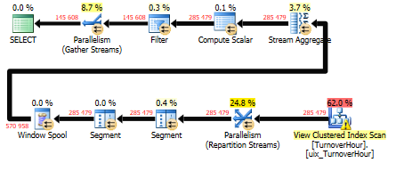
set dateformat ymd; create partition function pf_TurnoverHour(datetime) as range right for values ( '2006-01-01', '2006-02-01', '2006-03-01', '2006-04-01', '2006-05-01', '2006-06-01', '2006-07-01', '2006-08-01', '2006-09-01', '2006-10-01', '2006-11-01', '2006-12-01', '2007-01-01', '2007-02-01', '2007-03-01', '2007-04-01', '2007-05-01', '2007-06-01', '2007-07-01', '2007-08-01', '2007-09-01', '2007-10-01', '2007-11-01', '2007-12-01', '2008-01-01', '2008-02-01', '2008-03-01', '2008-04-01', '2008-05-01', '2008-06-01', '2008-07-01', '2008-08-01', '2008-09-01', '2008-10-01', '2008-11-01', '2008-12-01', '2009-01-01', '2009-02-01', '2009-03-01', '2009-04-01', '2009-05-01', '2009-06-01', '2009-07-01', '2009-08-01', '2009-09-01', '2009-10-01', '2009-11-01', '2009-12-01', '2010-01-01', '2010-02-01', '2010-03-01', '2010-04-01', '2010-05-01', '2010-06-01', '2010-07-01', '2010-08-01', '2010-09-01', '2010-10-01', '2010-11-01', '2010-12-01', '2011-01-01', '2011-02-01', '2011-03-01', '2011-04-01', '2011-05-01', '2011-06-01', '2011-07-01', '2011-08-01', '2011-09-01', '2011-10-01', '2011-11-01', '2011-12-01', '2012-01-01', '2012-02-01', '2012-03-01', '2012-04-01', '2012-05-01', '2012-06-01', '2012-07-01', '2012-08-01', '2012-09-01', '2012-10-01', '2012-11-01', '2012-12-01', '2013-01-01', '2013-02-01', '2013-03-01', '2013-04-01', '2013-05-01', '2013-06-01', '2013-07-01', '2013-08-01', '2013-09-01', '2013-10-01', '2013-11-01', '2013-12-01', '2014-01-01', '2014-02-01', '2014-03-01', '2014-04-01', '2014-05-01', '2014-06-01', '2014-07-01', '2014-08-01', '2014-09-01', '2014-10-01', '2014-11-01', '2014-12-01', '2015-01-01', '2015-02-01', '2015-03-01', '2015-04-01', '2015-05-01', '2015-06-01', '2015-07-01', '2015-08-01', '2015-09-01', '2015-10-01', '2015-11-01', '2015-12-01', '2016-01-01', '2016-02-01', '2016-03-01', '2016-04-01', '2016-05-01', '2016-06-01', '2016-07-01', '2016-08-01', '2016-09-01', '2016-10-01', '2016-11-01', '2016-12-01', '2017-01-01', '2017-02-01', '2017-03-01', '2017-04-01', '2017-05-01', '2017-06-01', '2017-07-01', '2017-08-01', '2017-09-01', '2017-10-01', '2017-11-01', '2017-12-01', '2018-01-01', '2018-02-01', '2018-03-01', '2018-04-01', '2018-05-01', '2018-06-01', '2018-07-01', '2018-08-01', '2018-09-01', '2018-10-01', '2018-11-01', '2018-12-01', '2019-01-01', '2019-02-01', '2019-03-01', '2019-04-01', '2019-05-01', '2019-06-01', '2019-07-01', '2019-08-01', '2019-09-01', '2019-10-01', '2019-11-01', '2019-12-01'); go create partition scheme ps_TurnoverHour as partition pf_TurnoverHour all to ([primary]); go : create unique clustered index uix_TurnoverHour on dbo.TurnoverHour (StorehouseID, ProductID, dt) with (data_compression=page) on ps_TurnoverHour(dt); --- 19 min , . : set dateformat ymd; declare @start datetime = '2015-01-02', @finish datetime = '2015-01-03' declare @start_month datetime = convert(datetime,convert(varchar(9),@start,120)+'1',120) select * from ( select dt, StorehouseID, ProductId, Quantity, sum(Quantity) over ( partition by StorehouseID, ProductID order by dt ) as Balance from dbo.TurnoverHour with(noexpand) where dt between @start_month and @finish ) as tmp where dt >= @start order by StorehouseID, ProductID, dt option(recompile); SQL Server running time:
CPU time = 7860 ms, elapsed time = 1725 ms.
SQL Server parse and compile time:
CPU time = 0 ms, elapsed time = 0 ms.
Request Plan Cost = 9.4
In fact, data in one section is selected and scanned by a cluster index rather quickly. It should be added here that when the request is parameterized, the unpleasant effect of parameter sniffing occurs, the option (recompile) is treated.
Source: https://habr.com/ru/post/330070/
All Articles