Solving the traveling salesman problem using the nearest neighbor method in Python
Fast and simple algorithm requiring modification
Among the methods of solving the traveling salesman problem, the nearest neighbor method attracts with the simplicity of the algorithm. The nearest neighbor method in the original formulation is to find a closed curve of minimal length connecting a given set of points on the plane [1]. My attention was attracted by the most common implementation of this algorithm in the Mathcad package, placed on the network on a resource [2]. The implementation itself is not very convenient, for example, it is impossible to derive a matrix of distances between points or analyze alternative routes.
On the resource [2] the following is quite fair criticism of this method. “The route is not optimal (not the shortest) and strongly depends on the choice of the first city. In fact, the traveling salesman problem has not been solved, but one Hamiltonian chain of the graph has been found. ” In the same place the way of some improvement of the nearest neighbor method is proposed. “The next possible optimization step is“ untiing the loops ”(eliminating crosshairs). Another solution is to enumerate all cities (graph tops) as the beginning of the route and select the shortest of all routes. ” However, the implementation of the last sentence is not given. Considering all these circumstances, I decided to implement the above algorithm in Python and at the same time provide for the possibility of choosing the starting point by the criterion of the minimum route length.
Program code with generation of random values of point coordinates
#!/usr/bin/env python #coding=utf8 import matplotlib.pyplot as plt import numpy as np from numpy import exp,sqrt n=50;m=100;ib=3;way=[];a=0 X=np.random.uniform(a,m,n) Y=np.random.uniform(a,m,n) #X=[10, 10, 100,100 ,30, 20, 20, 50, 50, 85, 85, 75, 35, 25, 30, 47, 50] #Y=[5, 85, 0,90,50, 55,50,75 ,25,50,20,80,25,70,10,50,100] #n=len(X) M = np.zeros([n,n]) # for i in np.arange(0,n,1): for j in np.arange(0,n,1): if i!=j: M[i,j]=sqrt((X[i]-X[j])**2+(Y[i]-Y[j])**2)# else: M[i,j]=float('inf')# way.append(ib) for i in np.arange(1,n,1): s=[] for j in np.arange(0,n,1): s.append(M[way[i-1],j]) way.append(s.index(min(s)))# for j in np.arange(0,i,1): M[way[i],way[j]]=float('inf') M[way[i],way[j]]=float('inf') S=sum([sqrt((X[way[i]]-X[way[i+1]])**2+(Y[way[i]]-Y[way[i+1]])**2) for i in np.arange(0,n-1,1)])+ sqrt((X[way[n-1]]-X[way[0]])**2+(Y[way[n-1]]-Y[way[0]])**2) plt.title(' -%s. -%i. -%i.\n X,Y %i %i'%(round(S,3),ib,n,a,m), size=14) X1=[X[way[i]] for i in np.arange(0,n,1)] Y1=[Y[way[i]] for i in np.arange(0,n,1)] plt.plot(X1, Y1, color='r', linestyle=' ', marker='o') plt.plot(X1, Y1, color='b', linewidth=1) X2=[X[way[n-1]],X[way[0]]] Y2=[Y[way[n-1]],Y[way[0]]] plt.plot(X2, Y2, color='g', linewidth=2, linestyle='-', label=' \n ') plt.legend(loc='best') plt.grid(True) plt.show() As a result, the program will receive.
')
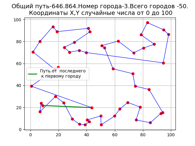
Disadvantages of the method are visible on the graph , as evidenced by the loop. The implementation of the algorithm in Python has more features than in Mathcad. For example, you can print a matrix of distances between points to print. For example, for n = 4, we get:
[[ inf 43.91676312 48.07577298 22.15545245] [43.91676312 inf 54.31419355 21.7749088 ] [48.07577298 54.31419355 inf 46.92141965] [ 22.15545245 21.7749088 46.92141965 inf]] For the operation of the algorithm on the main diagonal of the matrix, numerical values are set to infinity.
From the random coordinates of the points go to the given. The data will take on the resource [2]. To run the program in the mode of specified coordinates in the listing, remove the comments from the following lines.
X=[10, 10, 100,100 ,30, 20, 20, 50, 50, 85, 85, 75, 35, 25, 30, 47, 50] Y=[5, 85, 0,90,50, 55,50,75 ,25,50,20,80,25,70,10,50,100] n=len(X) As a result, the program will receive robots.
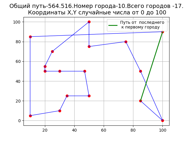
From the above graph, it can be seen that the traveling salesman’s trajectories intersect.
Comparison of algorithm implementations
To compare the results of my program with the program on the resource [2], we set the same parameters on the resource, with the only difference that my numbering of points (cities) starts from 0, and on the resource from 1. Then the city number on the resource n = 11, we get:
The length of the route 564, 516 and the location of the points are completely the same.
Neighbor Neighborhood Improvement
Now you can modify my program according to the criterion of the minimum length of the route.
The program code for determining the starting point from the condition of the minimum length of the marrut (modified algorithm).
#!/usr/bin/env python #codi import matplotlib.pyplot as plt import numpy as np from numpy import exp,sqrt n=50;m=100;way=[];a=0 X=np.random.uniform(a,m,n) Y=np.random.uniform(a,m,n) X=[10, 10, 100,100 ,30, 20, 20, 50, 50, 85, 85, 75, 35, 25, 30, 47, 50] Y=[5, 85, 0,90,50, 55,50,75 ,25,50,20,80,25,70,10,50,100] n=len(X) RS=[];RW=[];RIB=[] s=[] for ib in np.arange(0,n,1): M = np.zeros([n,n]) for i in np.arange(0,n,1): for j in np.arange(0,n,1): if i!=j: M[i,j]=sqrt((X[i]-X[j])**2+(Y[i]-Y[j])**2) else: M[i,j]=float('inf') way=[] way.append(ib) for i in np.arange(1,n,1): s=[] for j in np.arange(0,n,1): s.append(M[way[i-1],j]) way.append(s.index(min(s))) for j in np.arange(0,i,1): M[way[i],way[j]]=float('inf') M[way[i],way[j]]=float('inf') S=sum([sqrt((X[way[i]]-X[way[i+1]])**2+(Y[way[i]]-Y[way[i+1]])**2) for i in np.arange(0,n-1,1)])+ sqrt((X[way[n-1]]-X[way[0]])**2+(Y[way[n-1]]-Y[way[0]])**2) RS.append(S) RW.append(way) RIB.append(ib) S=min(RS) way=RW[RS.index(min(RS))] ib=RIB[RS.index(min(RS))] X1=[X[way[i]] for i in np.arange(0,n,1)] Y1=[Y[way[i]] for i in np.arange(0,n,1)] plt.title(' -%s. -%i. -%i.\n X,Y '%(round(S,3),ib,n), size=14) plt.plot(X1, Y1, color='r', linestyle=' ', marker='o') plt.plot(X1, Y1, color='b', linewidth=1) X2=[X[way[n-1]],X[way[0]]] Y2=[Y[way[n-1]],Y[way[0]]] plt.plot(X2, Y2, color='g', linewidth=2, linestyle='-', label=' \n ') plt.legend(loc='best') plt.grid(True) plt.show() Z=sqrt((X[way[n-1]]-X[way[0]])**2+(Y[way[n-1]]-Y[way[0]])**2) Y3=[sqrt((X[way[i+1]]-X[way[i]])**2+(Y[way[i+1]]-Y[way[i]])**2) for i in np.arange(0,n-1,1)] X3=[i for i in np.arange(0,n-1,1)] plt.title(' ') plt.plot(X3, Y3, color='b', linestyle=' ', marker='o') plt.plot(X3, Y3, color='r', linewidth=1, linestyle='-', label=' - %s'%str(round(Z,3))) plt.legend(loc='best') plt.grid(True) plt.show () The result of the program.
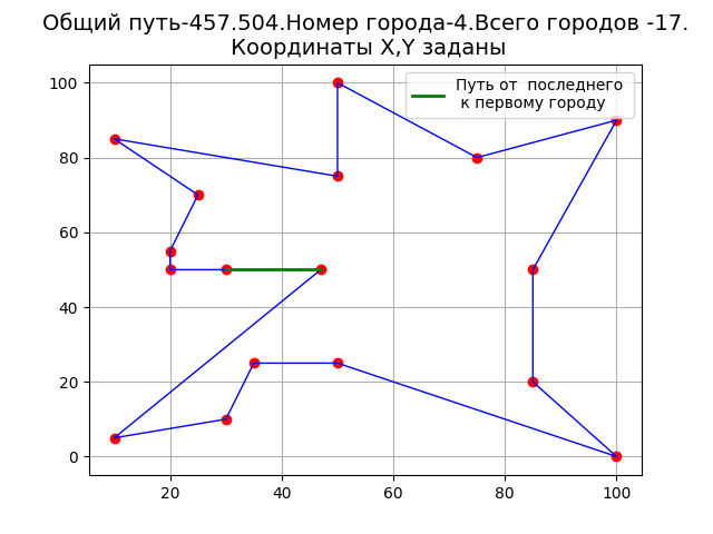
There are no loops on the graph, which indicates an improvement in the algorithm.

The length of the route at the beginning of movement from point 4 is less than at the beginning of movement from other points.
- 458.662, - 0 - 463.194, - 1 - 560.726, - 2 - 567.48, - 3 - 457.504, - 4 - 465.714, - 5 - 471.672, - 6 - 460.445, - 7 - 533.461, - 8 - 532.326, - 9 - 564.516, - 10 - 565.702, - 11 - 535.539, - 12 - 463.194, - 13 - 458.662, - 14 - 457.504, - 15 - 508.045, - 16 Dependence of the length of the route on the number of points (cities)
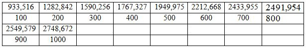
To do this, let's return to the generation of random coordinate values. According to the results of the program, increasing the number of points to 1000 steps in 100 we will make a table of two lines, in one length of routes to another number of points in a route.
We approximate the data with the help of the program.
#!/usr/bin/env python #coding=utf8 import matplotlib.pyplot as plt def mnkLIN(x,y): a=round((len(x)*sum([x[i]*y[i] for i in range(0,len(x))])-sum(x)*sum(y))/(len(x)*sum([x[i]**2 for i in range(0,len(x))])-sum(x)**2),3) b=round((sum(y)-a*sum(x))/len(x) ,3) y1=[round(a*w+b ,3) for w in x] s=[round((y1[i]-y[i])**2,3) for i in range(0,len(x))] sko=round((sum(s)/(len(x)-1))**0.5,3) p=(sko*len(x)*100)/sum(y1) plt.title(' \n Y=%s*x+%s -%i -.'%(str(a),str(b),int(p)), size=14) plt.xlabel(' ', size=14) plt.ylabel(' ', size=14) plt.plot(x, y, color='r', linestyle=' ', marker='o', label=' ') plt.plot(x, y1, color='b',linewidth=1, label=' ') plt.legend(loc='best') plt.grid(True) plt.show() y=[933.516, 1282.842, 1590.256, 1767.327 ,1949.975, 2212.668, 2433.955, 2491.954, 2549.579, 2748.672] x=[100,200,300,400,500,600, 700,800, 900,1000] mnkLIN(x,y) We get.

When using the nearest neighbor method, the route length and the number of points are related by a linear dependence in the given range. In [3], the analysis of the main methods of solving the traveling salesman problem was carried out. According to the data presented, the best results were shown by the Little algorithm, the genetic algorithm and the modification of the “go into the nearest” algorithm. This is an additional reason for the analysis of the traveling salesman problem solution in this article using the nearest neighbor method.
findings
Python is known to be a freely available programming language. I did not find any implementations of the nearest neighbor method in Python available to me. The simple implementation of the method proposed by me is certainly far from perfect, but it allows analyzing all the steps of the method - creating a matrix of distances between points, searching for a short route, modifying the algorithm, and features of a graphical display of route search results. All these are important factors especially in the learning process, when special mathematical packages are not available for understandable reasons. Therefore, I hope that my puny attempts to do without expensive mathematical packages for at least individual tasks will contribute not only to the rational organization of training, but also to the popularization of the Python programming language.
Thanks to everyone who reads the article and, perhaps, will use the results.
Links
Source: https://habr.com/ru/post/329604/
All Articles