Using statistics in PostgreSQL to optimize performance - Alexey Ermakov
Friends, we continue to publish transcriptions of the most interesting technical reports of past PG Day Russia conferences. Today, your attention is invited to the report of Alexei Yermakov , a specialist of Data Egret, dedicated to the device and the functioning of the scheduler.

The statistical information collected by PostgreSQL has a big impact on system performance. Knowing the statistics of data distribution, the optimizer can correctly estimate the number of rows, the required memory size, and select the fastest query execution plan. But in some rare cases, he may be wrong, and then DBA intervention is required.
')
In addition to information about the distribution of data, PostgreSQL also collects statistics on accessing tables and indexes, function calls, and even calls to individual queries (using the pg_stat_statements extension). This information, unlike distributions, is more needed by administrators than for the operation of the base itself, and it helps a lot to find and fix bottlenecks in the system.
The report will show how statistical information is collected, why it is important, and how to read and use it correctly; which parameters can be “tweaked” in certain cases, how to choose the optimal index and how to rewrite the query in order to correct the errors of the scheduler.
The report consists of two parts:
The first part is very theoretical. Let's see how the scheduler works, how statistics are collected and why, let us recall a little bit the theory of probability.
The second part will be more practical: why the scheduler sometimes mows down, which rakes and how they can be bypassed, and in the end there will be monitoring (how to understand that we have some problems with the base and what they are for).

How is the query in PostgreSQL? First, the application establishes a connection with PostgreSQL, sends the request body directly using the connection pool (pgbouncer, etc.). Further this request is parsed to tokens and broken into pieces. The tree is built, transferred to the rewrite system, and then the most interesting part is the planner / optimizer . In this place, we generate a query plan.
The scheduler can perform the same query in a bunch of different ways, and the more tables we have, the more ways we will get, this dependence grows as a factorial. Five tables - this is, let's say, some kind of constant 120, 10! - it will be a very large number. That is, we have a lot of plans, if we have a lot of tables, so you shouldn’t do queries with 20 join-s that a person cannot read normally, and the scheduler will be stupid at this point, and not will be able to choose the most optimal plan.
So, we got the plan, then we send it to the executor, which the plan executes step by step and then generates the result to the client.

Many execution plans are generated. For each such elementary operation (reading data from a table, sorting, combining results), the number of rows and the execution time in abstract parrots are estimated.

Create a test case. Suppose we have an abstract news site, on this site we have news and each news has a category, a numerical rating, and a content field with text.
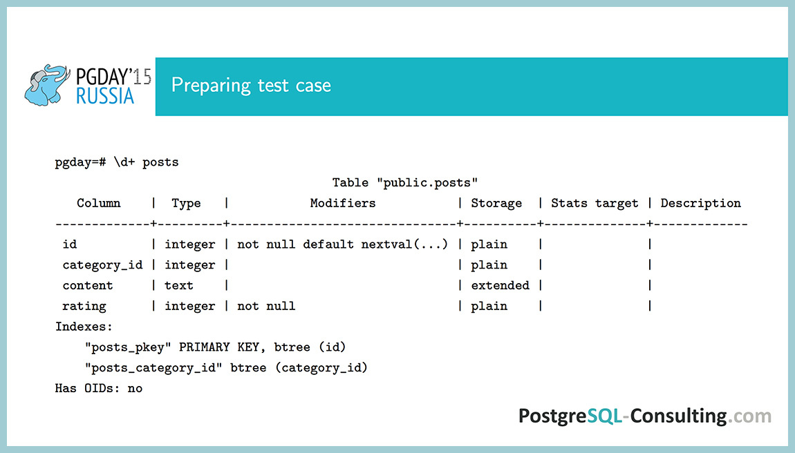
Let's see what happened: the \ d command shows information about the object in psql . We see a lot of interesting things: what indexes, what fields, what attributes, in general, all that was expected.

Now fill this table with test data. The id category field will be numbers from 0 to 99 that occur with the same probability. The content field will be the word "hello world", and at the end we will add the numeric indicator id to it. And our rating will be a normal distribution with a mathematical expectation of 50 and a standard deviation of 10. We will generate 10,000 such records.

That's what happened. Rating is a number about 50, category_id is integers and content field.

Let's see the COUNT query execution plan. Obviously, sequence scan, sequential reads. What interests us is the number of lines (10,000). How did the scheduler know that we have 10,000 lines? Just created a table, filled it, and the scheduler already knows.

There is a system table pg_class , which stores information about each table. It has two such advantageous fields: reltuples (the number of rows in this table) and relpages (the number of pages this table occupies). These numbers are not relevant, they are recorded in three cases:
It seems to be good that we have some meanings, but they may not be relevant. What to do in this case? We would like to have actual values. The scheduler in the application cannot quickly calculate the number of rows in a table (because it needs to read them all), but it can quickly count the number of pages that this table occupies. And, assuming that the number of lines on the page almost did not change after auto-vacuum or analyze , with the help of this proportion you can estimate the number of lines quite accurately. Why 10,000? After I recorded the data, the auto-analyze process went through (you can see this in the pg_stat_user_tables table, it keeps all sorts of monitoring counters).

Why did the auto-analyze process start at all, and what does it do? It is launched if the sum of the inserted, updated and deleted lines exceeds a certain threshold value. The threshold value is calculated based on two parameters:
10 percent is pretty good, but sometimes it's worth reducing it a little, in some difficult cases. For example, the table in which we store the queue: there are now 5 records in it, and a minute later it is already a million, then it is desirable to update the statistics more often.
Another parameter that auto-analyze has is default_statistics_target . It indicates how many pages and lines we take from the table, and also affects a number of other parameters, which will be discussed later. By default, this parameter is 100. What does auto-analyze do? He reads 300 * stats_target pages, and from these pages he selects 300 * stats_target lines. In total, by default, it will read 30,000 rows from a table and, based on this data, populate the pg_statistic table.

This table is not very convenient to read, so we came up with view pg_stats , which contains the same, but in a more readable format. What do we have here? One line of this view represents information about one field in the table. There is a field tablename, attname (table name, field name), and then the most interesting begins:

We created tables, let's see what was written after analyze for the ID field. We see that null_frac is zero, i.e. all values in the table are NOT NULL, because this is the primary key, and it is always NOT NULL. The average length is 4 (integer), n_distinct is -1. Why is -1, not ten thousand?
n_distinct can be either greater than zero or less than zero. If it is greater than zero, it shows the number of different values, and if less than zero, it shows a fraction of the number of lines that will take different values. That is, suppose if it were -0.5, then this would mean that half of the lines we have contain a unique value, and the second half contains their duplicates. In this case, it is -1, that is, all values are different.
In this case, the most_common_vals and most_common_freqs fields are empty, because all of the values we meet with the same probability, and there is no such that they are more common than others. And histogram_bounds contains 100 intervals. most_common_vals , most_common_freqs and histogram_bounds are set by the parameter default_statistics_target . In this case, it is 100 intervals and 100 different values can be stored maximum.
The last field is a correlation . This is a statistical term indicating whether there is a linear relationship between two random variables. In this case, there is a correlation between the value of the field and its physical position on the disk. This parameter can take values from -1 to 1. Take an example. The correlation between random variables as a person's height and weight, what will it be? Most likely, it will be more than zero. This shows that with increasing growth in our country, most likely the weight will also grow. Of course, not a fact, but it can be. If it were less than zero, then you would have an inverse relationship - with increasing growth, your weight would decrease. And if it were zero, it would mean that these things are most likely independent, that is, with any increase there can be any weight.

How is the selectivity of different conditions calculated? The query SELECT COUNT (*) , where ID <250. The Index Only Scan plan is selected, and we see that 250 rows are extracted. Why 250? Since we have no values in the most_common_vals and most_common_freqs array that are more common than others, the scheduler takes information from histogram_bounds . Once again, the probability of getting into each interval is about the same. By this criterion, he was created. The scheduler looks at how many intervals fall under this condition. Under it gets the first interval (from 1 to 100), the second interval (from 100 to 200) and half of the third. That is two and a half intervals. And in total there are 100 such intervals, and, thus, dividing 2.5 by 100, we get a selectivity of 2.5%. This is the percentage of lines that satisfy this condition. The number 100 is obtained as selectivity multiplied by cardinality. Cardinality is the total number of lines, I have already said how it counts. We get 2.5% of 10 thousand, that is 250 lines.

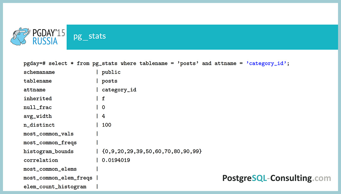
Now such an example. The CategoryID field: for it n_distinct is 100, that is, in this field we recorded numbers from zero to 99, which are evenly distributed. Here we see that histogram_bounds is empty, but the most_common_vals and most_common_freqs arrays are completely filled. The numbers in them are sorted by frequency, that is, the most popular value in this table is 98, which occurs in 1.21% of cases. The correlation here is at level 0, that is, all the data here are evenly mixed on the disk, there is no such that 1 is stored at the beginning of the table, and 99 is at the end of the table. We have a total of 100 values, and our default_statistics_target is also 100, so all the values we have fit here. If it didn’t fit, which will be in the following example, it will be different there.

How, in this case, is the selectivity calculated for the condition CategoryID = 98? Just given the value of the most_common_vals . If we have such a value, then we simply take the corresponding frequency and consider it to be equal to selectivity . In this case, we have 121 lines selected.

Now let's try changing the default_statistics_target for this field. We put it 10, although by default we had 100. Let's analyze . The \ d + command also shows, among other things, the stats_target value, if we changed it. That's what we did.
Now we have the most_common_vals and most_common_freqs are empty, but now we have the histogram_bounds field. How is selectivity calculated in this case?

According to this formula. That is, we can have either null or most_common_vals or histogram_bounds . In the numerator there is a probability that the value will be histogram_bounds , and in the denominator we have a number of different values, except for those already in most_common_vals . sumcommon is the sum of all values from the most_common_freqs array. This is not an obvious formula, but if you look at it, it’s clear why this works that way. Different values are distributed evenly across the histogram_bounds array. Although we get a selectivity of 1%, and this is a different estimate, in a hundred lines instead of 121. But 100 or 121 - in this case, this is not a problem, even if we have a half-order value, this is a good estimate.

Now let's see when we have two conditions: CategoryID = 98 and id <250 , that is, we combine two conditions. Selectivity is considered here as a product of selectivity, that is, according to a formula from probability theory: the probability that two events occur at the same time is equal to the probability that the first event will occur, multiplied by the probability that the second event will occur. This definition of statistical dependence, that is, it is assumed that these columns do not depend on each other. In this case, it is that they are independent of each other. It turns out a fair estimate, 2.5 lines. We discard the fractional part and get 2 lines. But realistically, 2.5 lines is also a good estimate.
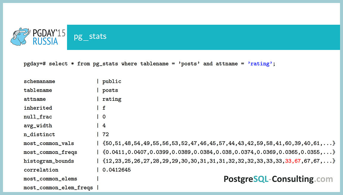
As a demonstration, let's see how the uneven distribution in the rating field looks. Both most_common_vals , and most_common_freqs , and even a histogram are filled in here . This should be enough to understand that the data here is uneven. Why is that? If they were evenly distributed, then the probability for each value would be one 1/72, that is, about 1%. We see that there are values with a probability of about 4%. Noticeably uneven distribution.

In addition to collecting information about the distribution of individual fields, information about the distribution of functional index values is also collected. This is not documented, there is no such information anywhere, access to this information is also not very convenient. If instead of tablename we put the name of the functional index, we get information about what is stored in it.
Suppose you create an index that stores the value of a rating in a square. Of course, there is no benefit from this, just as a demonstration to understand. If we compare this with the previous one, we will see that the value is simply squared. That is, if it was 50, then it became 2500. And histogram_bounds , respectively, will also be squared.
There is still such an undocumented thing, how to change statistics_target for a functional index: ALTER INDEX ALTER COLUMN ... set statistics - for some reason this is also not in the ALTER INDEX documentation.

Before that, there were examples where we compared a number with some constant, the CategoryID is equal to 98. And if we do not have a constant, but a subquery or the result of a function, what then to do with it? The scheduler assumes that there are some default estimators , that is, it simply takes the value of selectivity in the form of a constant. The probability that the field is equal to something, most likely, somewhere 0.5%. And the probability that something less than something will be somewhere around 33%. When we compare one column with another, this can also be.

As an example: ID <Select 100 . There is no information, so the number of rows is estimated at one third, that is, selectivity = 0.33 (3).

Everything that I am talking about can be viewed with hands, queries, without going to pg_stats. We look at the number of rows as SELECT COUNT (*), the number of rows with different CategoryID — as SELECT COUNT (DISTINCT category_id).

This is all good, but we cannot look at it in large tables. It will take a long time.

SELECT COUNT (*) on a table of several gigabytes is already very slow, and if you still do groupings, then very slowly. If we need more than one field, but several, it is worth looking at pg_stats. More convenient format and more information.
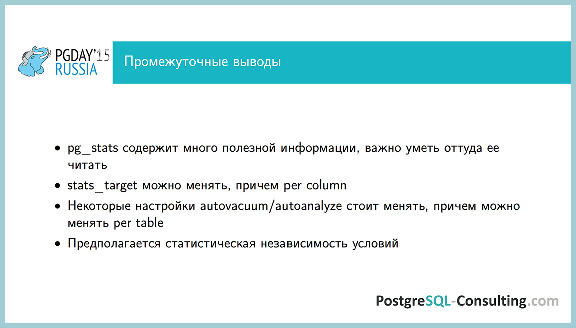
A lot of useful information is in pg_stats, stats_target can be changed for individual columns in the tables, the autovacuum and autoanalyze settings can be changed for individual tables, and here the statistical independence of conditions is manifested. If we have several conditions, they are considered independent, because there is no other information.

All this is good, but why is it necessary? If we had a perfect planner, we would not need anything of this, everything would work for us, the plan would always be optimal. But our planner is not perfect, and sometimes you have to go into it and see what you can do about it.

There is a useful technique : the foo table, 73GB, is very large, the number of rows can be viewed in reltuples . It turns out that it has 73 million lines.

We have a query: SELECT * FROM foo WHERE bar_id = 183 , you need to select the last 20 records from them. If we had a table of posts, it would be necessary to select 20 news of a certain category, for example. Very typical request. The n_distinct = 50 field, that is, 50 different values, and we have 70 million lines in total. And we see that the number 20 occurs in 55% of cases. That is, the distribution is extremely uneven. You can put the index on (bar_id, id) , it will work here, but the table is 73 GB. It turns out that this index may well occupy 5-7 GB. I do not really want to create such an index.

If we look, then 4 values account for 88% of the records. Such a thought arises: “Or maybe I should throw them out of the index? Why are they needed there? We will have an index 10 times less. ”
Take and discard these four bar_id values in part from the index. The size of the index was 758 MB. For all values that are not included in these 4, it will work for us, and everything will be very quickly executed.
A question from the audience : what if the parameters for excluding bar_id change?
If we know that we have such very frequent meanings, then we can “hard-code”. And if this does not happen, that today we have a distribution, and tomorrow it is the opposite, then this does not fit obviously. This is suitable for this case, when we know that our table is slowly growing, and if something does not work, then we will notice it. That is, we will see that the index will grow.
So, the index works for all values except four. It turns out that we do not need him.If we have a value of 20 in each second line, then we simply take the index on the primary key, read the last 40 lines and, most likely, 20 of them will be the ones we need. And in the worst case, we consider not 40 lines, but 200 or even 2000. But this is nonsense, counting 2000 lines by index is not a problem. Thus, we have disassembled this case.

More such an abstract case. Suppose we have conditions: a is equal to some value and bequal to no one value, and we think how to create an index? You can create an index on the field a, on the field b. You can create two indexes or an index in the a and b fields simultaneously, or in reverse order. You can create a partial index of a, where b is equal to something. Or maybe we don't need an index at all. How can you understand what index is needed for this query?

It is necessary to look, with what parameters it is caused. If we have enabled request logging, we can catch the slowest ones. We can look, with what parameters they were caused, what distributions are on these values. Knowing with what parameters the request is called, what distributions we have in this data, we can estimate the selectivity of each of these conditions. It will be different for each value, but, on average, it may be constant.
If there is a condition with a small selectivity (in this case, it is the percentage of rows that satisfies this condition), then we take it and set an index. If there is another condition with a small selectivity, we can set both indices if we lack one field. But if the selectivity is large (the boolean type field, which is false in 90% of cases), then we probably don’t need an index for it. And if it is needed, then we will do some partial index, most likely, in order not to drag these 90% in the index, there will be no benefit from them.

What are all the rakes with the scheduler ... The
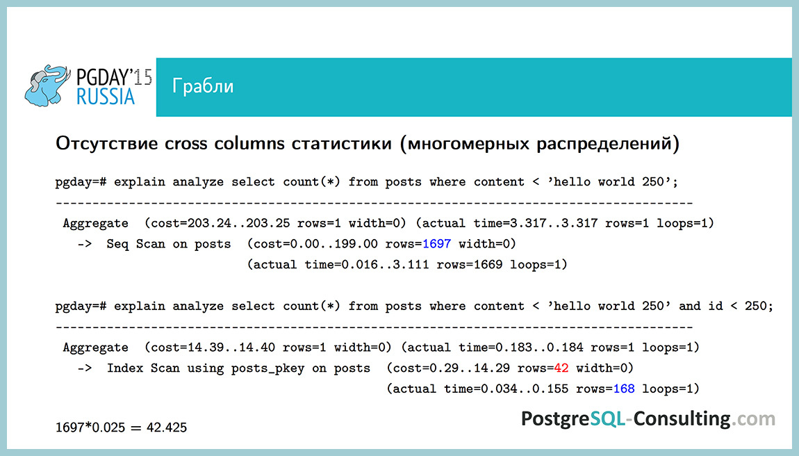
scheduler does not always work perfectly. For example, we do not have cross column statistics. We do not store information about the dependence of one field on another. As an example, considercontent <'hello world 250' . The condition is not very pleasant. We have 1600 lines selected, a sequential scan is obtained. And if we make two conditions: one of them is the same, and the second is id <250 , then the estimate differs by half a row: 142 lines versus 1697 lines. This is not very bad. If we had not two conditions, but three, which depend on each other, or the selectivity was smaller, the estimate may differ by many orders of magnitude.

This is a problem that is difficult to get around in a good way. You can somehow “zakhachit”, use the information that there is a default estimator, which will return us an estimate of 1/3 of all the lines, and here it is to screw it up. It is not recommended to do it all the time, but sometimes it can be done if nothing else can be done.
Here the id field is taken and added to it by abs (id) <0 . What does this mean?This condition is obviously false, abs is the modulus of the number, and the modulus of the number cannot be less than zero. This condition is always false, it does not affect the result, but it does affect the plan. The score here will increase by about one third for this condition, and the plan will be a little better. You can combine such hacks, use knowledge of default estimators. Perhaps you can come up with a better one, but in this case it turned out more or less normal.
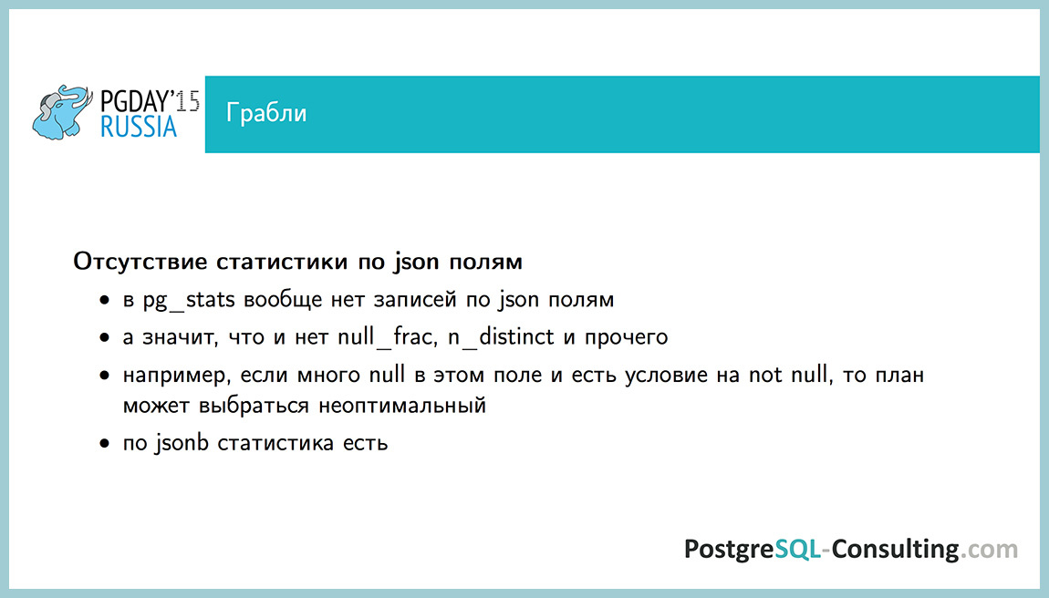
Next problem: no statistics for JSON fields. There is no information on this field in the pg_stats table. If we have some condition with this field, where it is NULL, or JOIN is done on it, the scheduler does not know anything about it, the plan may not be entirely optimal. You can use the JSONB field, everything is there.

The following rake - intarray operatorsDo not use statistics. Let's create a test table, in which we will write an array, in which the same value in each row: 100. If we look at the execution plan for the query “does the value 100 enter this array,” then we see that everything is fine, all the rows have been selected and the plan shows everything correctly.

But, if we create an extension intarray and execute the same query, it turns out that the default estimator is used and it selects 0.1% from us. Sometimes you can step on it, if such operators are used and there is an intarray, then the estimate may not be very good.
Fedor Sigaev, from the audience : I will comment, can I? This week there was a “patch” patch that cures this problem, but, unfortunately, it will only be in 9.6.

While this patch is not, you can somehow get around this. intarray rewrites the operator, replaces it with its own. If we use the post-statement operator in this case, then everything will work for us using the usual index without intarray.

The next problem is when we lack statistics_target. Suppose there are large tables that store a small number of different elements. In this case, the assessment of some rare element (which may not even be) may differ by several orders of magnitude. I already talked about this about this formula, she believes that all the remaining values are evenly distributed, but usually it is not. In this case, we can unscrew the statistics up to 10,000 or up to 1,000. There are artifacts, of course. Analyze on this table will work slower and the plan will be built a little slower, but sometimes this has to be done. For example, when join goes on several tables and there is not enough statistics.

The last part is about monitoring.. I talked about statistics on distributions (collected by the auto analyze process). In addition, the auto collector process collects statistics on all counters. There are quite a lot of interesting things here, I recommend to look into all the "views" pg_stat_ * . About some of them will tell.
pg_stat_user_tables- I already spoke about it, one line represents information on one table. What is interesting in it? How many sequence scans were on this table, how many scans selected rows, how many index scans were there, how many index scans did they select, when was the last autovacuum and autoanalyze, how many were there. There are also the number of records inserted, the number of records deleted, the number of live records. It seems, why is this necessary? Suppose if a table has a large number of rows that are extracted using sequence scan, and the table itself is also large, then, most likely, it lacks an index. We have such a query in the repository, which shows the TOP tables for which we have the most scans, and we can understand where to add the index.
pg_stat_user_indexes- information on individual indexes is stored here. You can understand, say, how many times this index has been used. It is useful if we want to understand whether the index created by us is used, or we want to take and delete some extra indexes.
pg_stat_user_functions - information on function calls. For each function there are fields that show how many times it has been called, how long it took. It is useful to know if we use a lot of functions.

These are stat collector statistics from the moment of launch, and it is not reset by itself, even when restarted. It can be reset with the pg_stat_reset () command . She will simply reset all counters. Most likely, there will be no problems from this, but you can see how the picture has changed after you have changed something.
The configuration parameter track_io_timing shows whether to collect statistics on disk I / O. This is very useful for the next item about pg_stat_statements, I’ll show you about it later. By default it is turned off, it is necessary to turn it on, but first check overhead, the documentation says how to do it.
Track_functions can be enabled to collect statistics on pg_stat_user_functions function calls. Another such case, if we have a lot of tables or a lot of databases, then there can be a lot of statistics, and the stats collector writes it directly to the file, this constant disk load on the record is not very useful. We can render stats_temp_directoryon a ramdisk, and then it will be written to memory. When you turn off the program, it simply writes to this directory. If there is an emergency shutdown, we will lose statistics, but there will be nothing terrible about it.
The track_activity_query_size field tells how long requests are collected in pg_stat_activity and pg_stat_statements. By default, 1024 bytes are collected from the request, sometimes it is worth raising it a little if we have long requests so that they can be read entirely.
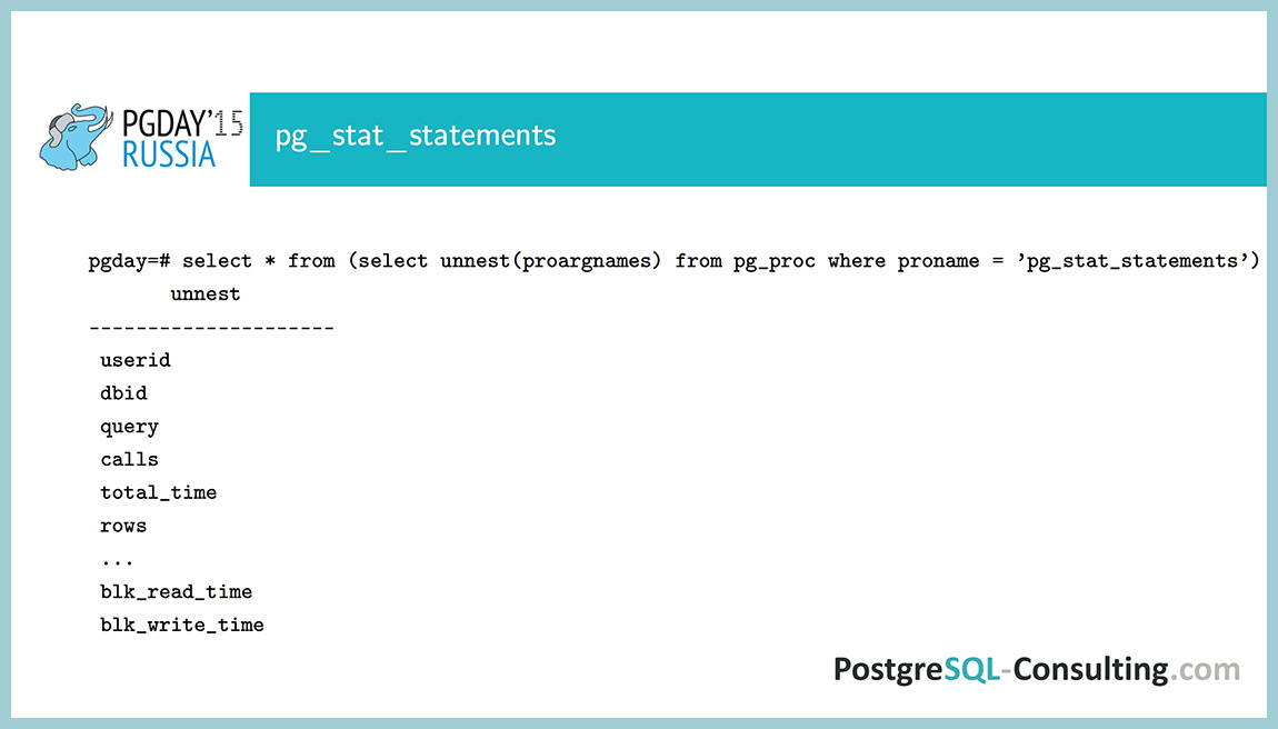
“Extension” pg_stat_statements, which collects all that is necessary. For some reason, they still don't use it. In fact, a very handy tool that collects information on the call of each request: how many times the request was called, how long it took to take, how many disk operations there were, how many rows were retrieved totally.

You can use specialized queries. We have made such a request, which accumulates a report, which states what generally happens in the database since the last reset of statistics. Real analyzed example, what do we see here?
In total, we performed requests for 50 hours, of which I / O took 0.6%. The very first request took the most time, it took 28% of the process time from the entire execution time in the program. A lot of useful information, very convenient. We are in the repository, it is called query_stat_total.sql , the link will continue.

These parameters are regulated by this. There are some parameters, you can read documentation about them, there is nothing complicated. Sometimes it is necessary to turn off track_utility, some system commands (all ORM or in Java, for example) like to add something to the deallocate request, and deallocate will have some new identifier every time, and here it will overwrite the values that we have in pg_stat_statements. It tracks only the TOP requests, by default it is one thousand requests (you can raise the value more), but if these requests are deallocate an identifier by 90%, then we will lose some information. In this case, you should turn off track_utility.

Conclusion: there are statistics on allocations, statistics on the use of resources, recorded by various processes, is also used in different ways. Statistics on distributions is used by the scheduler, and statistics on resources is hardly used by something, more for monitoring information.
Using these counters, you can identify bottlenecks, the scheduler can also be wrong, not a perfect world, is still being finalized, and pg_stat_statements should be used to monitor performance.

Some useful links to the manual, about estimating the number of lines by the scheduler, statistics collector, a cycle of articles depesz about how the scheduler works (five articles, and each one looks at how it works). Link to our repository and link to our blog.

Like the report of Alexei? Come visit us at PG Day'17 Russia ! Alexey will read the cognitive material about the features of the PostgreSQL scheduler device . We invite everyone who wants to know in detail how the planning of requests in the Posgres works. What ways can you influence the process of building a query execution plan? When should I try to force the scheduler to work correctly manually? Come , Alexey will tell everything :-)
The statistical information collected by PostgreSQL has a big impact on system performance. Knowing the statistics of data distribution, the optimizer can correctly estimate the number of rows, the required memory size, and select the fastest query execution plan. But in some rare cases, he may be wrong, and then DBA intervention is required.
')
In addition to information about the distribution of data, PostgreSQL also collects statistics on accessing tables and indexes, function calls, and even calls to individual queries (using the pg_stat_statements extension). This information, unlike distributions, is more needed by administrators than for the operation of the base itself, and it helps a lot to find and fix bottlenecks in the system.
The report will show how statistical information is collected, why it is important, and how to read and use it correctly; which parameters can be “tweaked” in certain cases, how to choose the optimal index and how to rewrite the query in order to correct the errors of the scheduler.
The report consists of two parts:
The first part is very theoretical. Let's see how the scheduler works, how statistics are collected and why, let us recall a little bit the theory of probability.
The second part will be more practical: why the scheduler sometimes mows down, which rakes and how they can be bypassed, and in the end there will be monitoring (how to understand that we have some problems with the base and what they are for).
How is the query in PostgreSQL? First, the application establishes a connection with PostgreSQL, sends the request body directly using the connection pool (pgbouncer, etc.). Further this request is parsed to tokens and broken into pieces. The tree is built, transferred to the rewrite system, and then the most interesting part is the planner / optimizer . In this place, we generate a query plan.
The scheduler can perform the same query in a bunch of different ways, and the more tables we have, the more ways we will get, this dependence grows as a factorial. Five tables - this is, let's say, some kind of constant 120, 10! - it will be a very large number. That is, we have a lot of plans, if we have a lot of tables, so you shouldn’t do queries with 20 join-s that a person cannot read normally, and the scheduler will be stupid at this point, and not will be able to choose the most optimal plan.
So, we got the plan, then we send it to the executor, which the plan executes step by step and then generates the result to the client.
Many execution plans are generated. For each such elementary operation (reading data from a table, sorting, combining results), the number of rows and the execution time in abstract parrots are estimated.
Create a test case. Suppose we have an abstract news site, on this site we have news and each news has a category, a numerical rating, and a content field with text.
Let's see what happened: the \ d command shows information about the object in psql . We see a lot of interesting things: what indexes, what fields, what attributes, in general, all that was expected.
Now fill this table with test data. The id category field will be numbers from 0 to 99 that occur with the same probability. The content field will be the word "hello world", and at the end we will add the numeric indicator id to it. And our rating will be a normal distribution with a mathematical expectation of 50 and a standard deviation of 10. We will generate 10,000 such records.
That's what happened. Rating is a number about 50, category_id is integers and content field.
Let's see the COUNT query execution plan. Obviously, sequence scan, sequential reads. What interests us is the number of lines (10,000). How did the scheduler know that we have 10,000 lines? Just created a table, filled it, and the scheduler already knows.
There is a system table pg_class , which stores information about each table. It has two such advantageous fields: reltuples (the number of rows in this table) and relpages (the number of pages this table occupies). These numbers are not relevant, they are recorded in three cases:
- the auto-vacuum process went through the table, read the table and updated the fields;
- the auto-analyze process went through the table, read all or part of the table and updated the same fields;
- we have created an index or have performed some other DDL operation on the table, in this case, all these fields can also be updated.
It seems to be good that we have some meanings, but they may not be relevant. What to do in this case? We would like to have actual values. The scheduler in the application cannot quickly calculate the number of rows in a table (because it needs to read them all), but it can quickly count the number of pages that this table occupies. And, assuming that the number of lines on the page almost did not change after auto-vacuum or analyze , with the help of this proportion you can estimate the number of lines quite accurately. Why 10,000? After I recorded the data, the auto-analyze process went through (you can see this in the pg_stat_user_tables table, it keeps all sorts of monitoring counters).
Why did the auto-analyze process start at all, and what does it do? It is launched if the sum of the inserted, updated and deleted lines exceeds a certain threshold value. The threshold value is calculated based on two parameters:
- fixed constant, which is set in the config or for a specific table via ALTER TABLE ( autovacuum_analyze_threshold , fixed part, it is 50 by default);
- autovacuum_analyze_scale_factor parameter: the proportion of rows in the table that, if changed, will start the analyze (by default, this is 0.1 or 10%).
10 percent is pretty good, but sometimes it's worth reducing it a little, in some difficult cases. For example, the table in which we store the queue: there are now 5 records in it, and a minute later it is already a million, then it is desirable to update the statistics more often.
Another parameter that auto-analyze has is default_statistics_target . It indicates how many pages and lines we take from the table, and also affects a number of other parameters, which will be discussed later. By default, this parameter is 100. What does auto-analyze do? He reads 300 * stats_target pages, and from these pages he selects 300 * stats_target lines. In total, by default, it will read 30,000 rows from a table and, based on this data, populate the pg_statistic table.
This table is not very convenient to read, so we came up with view pg_stats , which contains the same, but in a more readable format. What do we have here? One line of this view represents information about one field in the table. There is a field tablename, attname (table name, field name), and then the most interesting begins:
- null_frac tells us how the percentage of rows for this table is null;
- avg_width - the average length of the field in the table (for fields of fixed length, this field will not tell us anything);
- n_distinct shows how many different values are in this field;
- The most_common_vals and most_common_freqs arrays contain the most common field values and their corresponding frequencies;
- histogram_bounds is an array of intervals, and the probability of falling into each interval is approximately the same.
We created tables, let's see what was written after analyze for the ID field. We see that null_frac is zero, i.e. all values in the table are NOT NULL, because this is the primary key, and it is always NOT NULL. The average length is 4 (integer), n_distinct is -1. Why is -1, not ten thousand?
n_distinct can be either greater than zero or less than zero. If it is greater than zero, it shows the number of different values, and if less than zero, it shows a fraction of the number of lines that will take different values. That is, suppose if it were -0.5, then this would mean that half of the lines we have contain a unique value, and the second half contains their duplicates. In this case, it is -1, that is, all values are different.
In this case, the most_common_vals and most_common_freqs fields are empty, because all of the values we meet with the same probability, and there is no such that they are more common than others. And histogram_bounds contains 100 intervals. most_common_vals , most_common_freqs and histogram_bounds are set by the parameter default_statistics_target . In this case, it is 100 intervals and 100 different values can be stored maximum.
The last field is a correlation . This is a statistical term indicating whether there is a linear relationship between two random variables. In this case, there is a correlation between the value of the field and its physical position on the disk. This parameter can take values from -1 to 1. Take an example. The correlation between random variables as a person's height and weight, what will it be? Most likely, it will be more than zero. This shows that with increasing growth in our country, most likely the weight will also grow. Of course, not a fact, but it can be. If it were less than zero, then you would have an inverse relationship - with increasing growth, your weight would decrease. And if it were zero, it would mean that these things are most likely independent, that is, with any increase there can be any weight.
How is the selectivity of different conditions calculated? The query SELECT COUNT (*) , where ID <250. The Index Only Scan plan is selected, and we see that 250 rows are extracted. Why 250? Since we have no values in the most_common_vals and most_common_freqs array that are more common than others, the scheduler takes information from histogram_bounds . Once again, the probability of getting into each interval is about the same. By this criterion, he was created. The scheduler looks at how many intervals fall under this condition. Under it gets the first interval (from 1 to 100), the second interval (from 100 to 200) and half of the third. That is two and a half intervals. And in total there are 100 such intervals, and, thus, dividing 2.5 by 100, we get a selectivity of 2.5%. This is the percentage of lines that satisfy this condition. The number 100 is obtained as selectivity multiplied by cardinality. Cardinality is the total number of lines, I have already said how it counts. We get 2.5% of 10 thousand, that is 250 lines.
Now such an example. The CategoryID field: for it n_distinct is 100, that is, in this field we recorded numbers from zero to 99, which are evenly distributed. Here we see that histogram_bounds is empty, but the most_common_vals and most_common_freqs arrays are completely filled. The numbers in them are sorted by frequency, that is, the most popular value in this table is 98, which occurs in 1.21% of cases. The correlation here is at level 0, that is, all the data here are evenly mixed on the disk, there is no such that 1 is stored at the beginning of the table, and 99 is at the end of the table. We have a total of 100 values, and our default_statistics_target is also 100, so all the values we have fit here. If it didn’t fit, which will be in the following example, it will be different there.
How, in this case, is the selectivity calculated for the condition CategoryID = 98? Just given the value of the most_common_vals . If we have such a value, then we simply take the corresponding frequency and consider it to be equal to selectivity . In this case, we have 121 lines selected.
Now let's try changing the default_statistics_target for this field. We put it 10, although by default we had 100. Let's analyze . The \ d + command also shows, among other things, the stats_target value, if we changed it. That's what we did.
Now we have the most_common_vals and most_common_freqs are empty, but now we have the histogram_bounds field. How is selectivity calculated in this case?
According to this formula. That is, we can have either null or most_common_vals or histogram_bounds . In the numerator there is a probability that the value will be histogram_bounds , and in the denominator we have a number of different values, except for those already in most_common_vals . sumcommon is the sum of all values from the most_common_freqs array. This is not an obvious formula, but if you look at it, it’s clear why this works that way. Different values are distributed evenly across the histogram_bounds array. Although we get a selectivity of 1%, and this is a different estimate, in a hundred lines instead of 121. But 100 or 121 - in this case, this is not a problem, even if we have a half-order value, this is a good estimate.
Now let's see when we have two conditions: CategoryID = 98 and id <250 , that is, we combine two conditions. Selectivity is considered here as a product of selectivity, that is, according to a formula from probability theory: the probability that two events occur at the same time is equal to the probability that the first event will occur, multiplied by the probability that the second event will occur. This definition of statistical dependence, that is, it is assumed that these columns do not depend on each other. In this case, it is that they are independent of each other. It turns out a fair estimate, 2.5 lines. We discard the fractional part and get 2 lines. But realistically, 2.5 lines is also a good estimate.
As a demonstration, let's see how the uneven distribution in the rating field looks. Both most_common_vals , and most_common_freqs , and even a histogram are filled in here . This should be enough to understand that the data here is uneven. Why is that? If they were evenly distributed, then the probability for each value would be one 1/72, that is, about 1%. We see that there are values with a probability of about 4%. Noticeably uneven distribution.
In addition to collecting information about the distribution of individual fields, information about the distribution of functional index values is also collected. This is not documented, there is no such information anywhere, access to this information is also not very convenient. If instead of tablename we put the name of the functional index, we get information about what is stored in it.
Suppose you create an index that stores the value of a rating in a square. Of course, there is no benefit from this, just as a demonstration to understand. If we compare this with the previous one, we will see that the value is simply squared. That is, if it was 50, then it became 2500. And histogram_bounds , respectively, will also be squared.
There is still such an undocumented thing, how to change statistics_target for a functional index: ALTER INDEX ALTER COLUMN ... set statistics - for some reason this is also not in the ALTER INDEX documentation.
Before that, there were examples where we compared a number with some constant, the CategoryID is equal to 98. And if we do not have a constant, but a subquery or the result of a function, what then to do with it? The scheduler assumes that there are some default estimators , that is, it simply takes the value of selectivity in the form of a constant. The probability that the field is equal to something, most likely, somewhere 0.5%. And the probability that something less than something will be somewhere around 33%. When we compare one column with another, this can also be.
As an example: ID <Select 100 . There is no information, so the number of rows is estimated at one third, that is, selectivity = 0.33 (3).
Everything that I am talking about can be viewed with hands, queries, without going to pg_stats. We look at the number of rows as SELECT COUNT (*), the number of rows with different CategoryID — as SELECT COUNT (DISTINCT category_id).
This is all good, but we cannot look at it in large tables. It will take a long time.
SELECT COUNT (*) on a table of several gigabytes is already very slow, and if you still do groupings, then very slowly. If we need more than one field, but several, it is worth looking at pg_stats. More convenient format and more information.
A lot of useful information is in pg_stats, stats_target can be changed for individual columns in the tables, the autovacuum and autoanalyze settings can be changed for individual tables, and here the statistical independence of conditions is manifested. If we have several conditions, they are considered independent, because there is no other information.
All this is good, but why is it necessary? If we had a perfect planner, we would not need anything of this, everything would work for us, the plan would always be optimal. But our planner is not perfect, and sometimes you have to go into it and see what you can do about it.
There is a useful technique : the foo table, 73GB, is very large, the number of rows can be viewed in reltuples . It turns out that it has 73 million lines.
We have a query: SELECT * FROM foo WHERE bar_id = 183 , you need to select the last 20 records from them. If we had a table of posts, it would be necessary to select 20 news of a certain category, for example. Very typical request. The n_distinct = 50 field, that is, 50 different values, and we have 70 million lines in total. And we see that the number 20 occurs in 55% of cases. That is, the distribution is extremely uneven. You can put the index on (bar_id, id) , it will work here, but the table is 73 GB. It turns out that this index may well occupy 5-7 GB. I do not really want to create such an index.
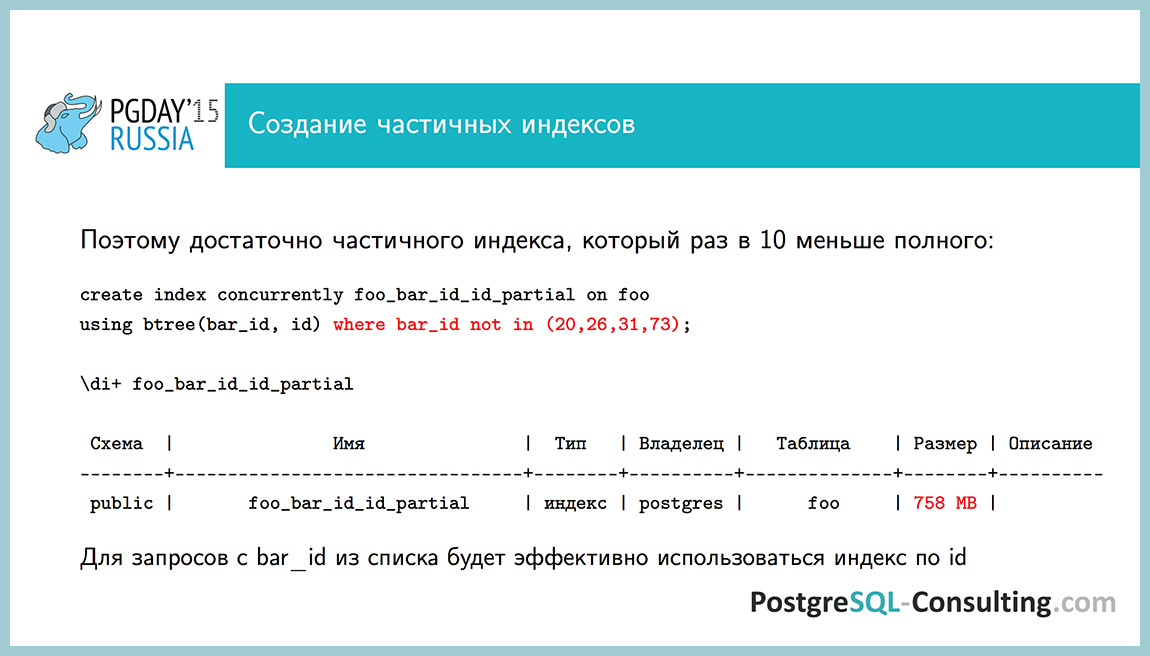
If we look, then 4 values account for 88% of the records. Such a thought arises: “Or maybe I should throw them out of the index? Why are they needed there? We will have an index 10 times less. ”
Take and discard these four bar_id values in part from the index. The size of the index was 758 MB. For all values that are not included in these 4, it will work for us, and everything will be very quickly executed.
A question from the audience : what if the parameters for excluding bar_id change?
If we know that we have such very frequent meanings, then we can “hard-code”. And if this does not happen, that today we have a distribution, and tomorrow it is the opposite, then this does not fit obviously. This is suitable for this case, when we know that our table is slowly growing, and if something does not work, then we will notice it. That is, we will see that the index will grow.
So, the index works for all values except four. It turns out that we do not need him.If we have a value of 20 in each second line, then we simply take the index on the primary key, read the last 40 lines and, most likely, 20 of them will be the ones we need. And in the worst case, we consider not 40 lines, but 200 or even 2000. But this is nonsense, counting 2000 lines by index is not a problem. Thus, we have disassembled this case.
More such an abstract case. Suppose we have conditions: a is equal to some value and bequal to no one value, and we think how to create an index? You can create an index on the field a, on the field b. You can create two indexes or an index in the a and b fields simultaneously, or in reverse order. You can create a partial index of a, where b is equal to something. Or maybe we don't need an index at all. How can you understand what index is needed for this query?
It is necessary to look, with what parameters it is caused. If we have enabled request logging, we can catch the slowest ones. We can look, with what parameters they were caused, what distributions are on these values. Knowing with what parameters the request is called, what distributions we have in this data, we can estimate the selectivity of each of these conditions. It will be different for each value, but, on average, it may be constant.
If there is a condition with a small selectivity (in this case, it is the percentage of rows that satisfies this condition), then we take it and set an index. If there is another condition with a small selectivity, we can set both indices if we lack one field. But if the selectivity is large (the boolean type field, which is false in 90% of cases), then we probably don’t need an index for it. And if it is needed, then we will do some partial index, most likely, in order not to drag these 90% in the index, there will be no benefit from them.
What are all the rakes with the scheduler ... The
scheduler does not always work perfectly. For example, we do not have cross column statistics. We do not store information about the dependence of one field on another. As an example, considercontent <'hello world 250' . The condition is not very pleasant. We have 1600 lines selected, a sequential scan is obtained. And if we make two conditions: one of them is the same, and the second is id <250 , then the estimate differs by half a row: 142 lines versus 1697 lines. This is not very bad. If we had not two conditions, but three, which depend on each other, or the selectivity was smaller, the estimate may differ by many orders of magnitude.
This is a problem that is difficult to get around in a good way. You can somehow “zakhachit”, use the information that there is a default estimator, which will return us an estimate of 1/3 of all the lines, and here it is to screw it up. It is not recommended to do it all the time, but sometimes it can be done if nothing else can be done.
Here the id field is taken and added to it by abs (id) <0 . What does this mean?This condition is obviously false, abs is the modulus of the number, and the modulus of the number cannot be less than zero. This condition is always false, it does not affect the result, but it does affect the plan. The score here will increase by about one third for this condition, and the plan will be a little better. You can combine such hacks, use knowledge of default estimators. Perhaps you can come up with a better one, but in this case it turned out more or less normal.
Next problem: no statistics for JSON fields. There is no information on this field in the pg_stats table. If we have some condition with this field, where it is NULL, or JOIN is done on it, the scheduler does not know anything about it, the plan may not be entirely optimal. You can use the JSONB field, everything is there.
The following rake - intarray operatorsDo not use statistics. Let's create a test table, in which we will write an array, in which the same value in each row: 100. If we look at the execution plan for the query “does the value 100 enter this array,” then we see that everything is fine, all the rows have been selected and the plan shows everything correctly.
But, if we create an extension intarray and execute the same query, it turns out that the default estimator is used and it selects 0.1% from us. Sometimes you can step on it, if such operators are used and there is an intarray, then the estimate may not be very good.
Fedor Sigaev, from the audience : I will comment, can I? This week there was a “patch” patch that cures this problem, but, unfortunately, it will only be in 9.6.
While this patch is not, you can somehow get around this. intarray rewrites the operator, replaces it with its own. If we use the post-statement operator in this case, then everything will work for us using the usual index without intarray.
The next problem is when we lack statistics_target. Suppose there are large tables that store a small number of different elements. In this case, the assessment of some rare element (which may not even be) may differ by several orders of magnitude. I already talked about this about this formula, she believes that all the remaining values are evenly distributed, but usually it is not. In this case, we can unscrew the statistics up to 10,000 or up to 1,000. There are artifacts, of course. Analyze on this table will work slower and the plan will be built a little slower, but sometimes this has to be done. For example, when join goes on several tables and there is not enough statistics.
The last part is about monitoring.. I talked about statistics on distributions (collected by the auto analyze process). In addition, the auto collector process collects statistics on all counters. There are quite a lot of interesting things here, I recommend to look into all the "views" pg_stat_ * . About some of them will tell.
pg_stat_user_tables- I already spoke about it, one line represents information on one table. What is interesting in it? How many sequence scans were on this table, how many scans selected rows, how many index scans were there, how many index scans did they select, when was the last autovacuum and autoanalyze, how many were there. There are also the number of records inserted, the number of records deleted, the number of live records. It seems, why is this necessary? Suppose if a table has a large number of rows that are extracted using sequence scan, and the table itself is also large, then, most likely, it lacks an index. We have such a query in the repository, which shows the TOP tables for which we have the most scans, and we can understand where to add the index.
pg_stat_user_indexes- information on individual indexes is stored here. You can understand, say, how many times this index has been used. It is useful if we want to understand whether the index created by us is used, or we want to take and delete some extra indexes.
pg_stat_user_functions - information on function calls. For each function there are fields that show how many times it has been called, how long it took. It is useful to know if we use a lot of functions.
These are stat collector statistics from the moment of launch, and it is not reset by itself, even when restarted. It can be reset with the pg_stat_reset () command . She will simply reset all counters. Most likely, there will be no problems from this, but you can see how the picture has changed after you have changed something.
The configuration parameter track_io_timing shows whether to collect statistics on disk I / O. This is very useful for the next item about pg_stat_statements, I’ll show you about it later. By default it is turned off, it is necessary to turn it on, but first check overhead, the documentation says how to do it.
Track_functions can be enabled to collect statistics on pg_stat_user_functions function calls. Another such case, if we have a lot of tables or a lot of databases, then there can be a lot of statistics, and the stats collector writes it directly to the file, this constant disk load on the record is not very useful. We can render stats_temp_directoryon a ramdisk, and then it will be written to memory. When you turn off the program, it simply writes to this directory. If there is an emergency shutdown, we will lose statistics, but there will be nothing terrible about it.
The track_activity_query_size field tells how long requests are collected in pg_stat_activity and pg_stat_statements. By default, 1024 bytes are collected from the request, sometimes it is worth raising it a little if we have long requests so that they can be read entirely.
“Extension” pg_stat_statements, which collects all that is necessary. For some reason, they still don't use it. In fact, a very handy tool that collects information on the call of each request: how many times the request was called, how long it took to take, how many disk operations there were, how many rows were retrieved totally.
You can use specialized queries. We have made such a request, which accumulates a report, which states what generally happens in the database since the last reset of statistics. Real analyzed example, what do we see here?
In total, we performed requests for 50 hours, of which I / O took 0.6%. The very first request took the most time, it took 28% of the process time from the entire execution time in the program. A lot of useful information, very convenient. We are in the repository, it is called query_stat_total.sql , the link will continue.
These parameters are regulated by this. There are some parameters, you can read documentation about them, there is nothing complicated. Sometimes it is necessary to turn off track_utility, some system commands (all ORM or in Java, for example) like to add something to the deallocate request, and deallocate will have some new identifier every time, and here it will overwrite the values that we have in pg_stat_statements. It tracks only the TOP requests, by default it is one thousand requests (you can raise the value more), but if these requests are deallocate an identifier by 90%, then we will lose some information. In this case, you should turn off track_utility.
Conclusion: there are statistics on allocations, statistics on the use of resources, recorded by various processes, is also used in different ways. Statistics on distributions is used by the scheduler, and statistics on resources is hardly used by something, more for monitoring information.
Using these counters, you can identify bottlenecks, the scheduler can also be wrong, not a perfect world, is still being finalized, and pg_stat_statements should be used to monitor performance.
Some useful links to the manual, about estimating the number of lines by the scheduler, statistics collector, a cycle of articles depesz about how the scheduler works (five articles, and each one looks at how it works). Link to our repository and link to our blog.
Like the report of Alexei? Come visit us at PG Day'17 Russia ! Alexey will read the cognitive material about the features of the PostgreSQL scheduler device . We invite everyone who wants to know in detail how the planning of requests in the Posgres works. What ways can you influence the process of building a query execution plan? When should I try to force the scheduler to work correctly manually? Come , Alexey will tell everything :-)
Source: https://habr.com/ru/post/329542/
All Articles