Autopilot on your own: sensor fusion from the phone and open training data

Hello. We continue to collect autopilot on computer vision from githubs and sticks ( start here ). Today we are connecting to the motion sensors of the smartphone (accelerometer, gyroscope and GPS receiver) on Android, we are developing an uncomplicated sensor fusion and finally closing it with the code to collect the training sample. Bonuses - Android application for recording all sensors synchronized with video and more than an hour of tagged data as part of import substitution of foreign contests . All code is still on github .

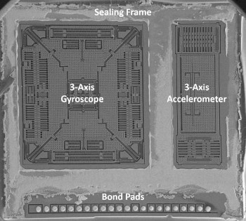
These are three-axis MEMS accelerometer and gyroscope, they will be extremely useful to us.

In a nutshell, I’ll remind you (for the details, welcome to the previous post that the ultimate goal is to train a system that will be able to give out control actions for the car (video steering angle and the desired speed or acceleration) by video frame from the windshield.) video from the races, where the machine is controlled by a man, and time-synchronized information about the angle of rotation and speed.In modern cars, this data can be read through the CAN bus , but first you need to buy and connect a special CAN adapter ter, and secondly, to deal with the decoding of the protocol and data format, which are different for different manufacturers. Instead of all this trouble, we calculate the control actions indirectly - from raw data from an ordinary smartphone, which is not connected to anything else.

In the last series, we learned how to determine the angular speed of a car turning in a horizontal plane based on only video frames using the video-SLAM library . Unfortunately, in practice this library very inaccurately calculates the translational speed of the device. And without knowing the translational speed, we cannot train even the steering component for the autopilot separately, since the angular velocity $\ omega$ depends on the combination of the degree of rotation of the steering wheel (equivalently, the turning radius ) and the forward speed of the car .

To get a forward speed, today we are switching from video processing to motion sensors, which almost any smartphone has: a GPS receiver, an accelerometer and a gyroscope. Let's look at the pros and cons of each, combine the information and get the instantaneous speed for each frame of video. Moreover, we will also take information about the rotations from the gyroscope, which will make it possible to abandon the more capricious optical SLAM and the calibration of the smartphone camera that it needs. As a result, the new process of collecting data dries up to three "button clicks": we put the application on the phone - we record the track on the race - we process it with one command on the computer.

As a result, we obtain a frame-by-frame annotation with the translational speed and the speed of turns:

Available motion sensors

We will work with android. Whatever the platform - for those who know English, an interesting video about how information from different sensors can complement calibration and reduce errors. We are interested in motion sensors (accelerometer and gyroscope) and location (GPS) sensors .

From the point of view of the API, everything is simple - we ask the user for permissions, subscribe for updates, and get a stream of events with a sensor reading and measurement time. Details can be found in the source .

Consider the pros and cons of sensors.

GPS

GPS is, as it turned out, 90% success in determining translational speed, at least in relatively open spaces. From GPS come in the Location format:

Estimation of the absolute position (latitude, longitude).
An estimate of the accuracy of the coordinates is the radius of the confidence circle of 68% around the estimate. That is, in ~ 68% of measurements, the present position of the device must be within the limits of a given radius around the estimate. As a rule, on more or less open space, the accuracy is within 3-4 meters.
Absolute speed (no direction), estimated from past measured GPS positions.

A huge plus of GPS data is that the measurement errors are independent , that is, they do not accumulate over time: the new measurement is not affected by how many measurements there were before that and the large errors. This is a very important feature on which the rest of the approach relies.

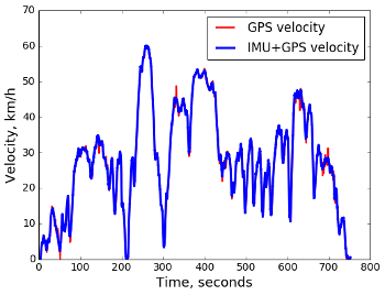
The disadvantage is that measurements are rarely taken , about 1 time per second, and there is no sense to carry them out much more often - the movement of the device would still be comparable to a measurement error. As a result, firstly, GPS data is late in reacting to a change in speed, and secondly, it is more difficult to remove noise from them — to do this, you need to look at the measurements that are next in time, which aggravates the time vagueness even more. Here is an example of a speed chart with GPS:

Here, the first 25 seconds (constant acceleration and probable delay of GPS measurements) and noise between 30 and 40 seconds are suspicious. For the seed, the same graph after processing data from the accelerometer and gyroscope:

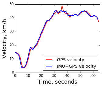
As you can see, there are improvements in both indicators: we react to accelerations earlier, and the outburst at 35 seconds is smoothed out.

Inertial sensors: accelerometer and gyroscope

Inertial sensors measure acceleration, linear (accelerometer) and centripetal (gyroscope). The result of their measurements is an estimate of the change in the movement of the device relative to the previous point in time. Mathematically, this is reflected in the use of a device-related coordinate system :

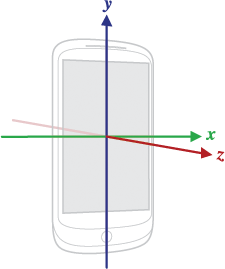
The accelerometer provides linear accelerations along the three axes of the device, the gyroscope - the angular velocity around the same three axes.

Plus inertial sensors - the possibility of very frequent measurements , at 400 Hz and above, which by an order of magnitude overlaps the frequency of video frames at ~ 30 Hz. The main disadvantage is the lack of communication with a fixed coordinate system. The sensors are capable of measuring only the change relative to the previous position, therefore, to calculate the results in a fixed coordinate system, their readings need to be integrated over time, and the measurement errors accumulate - the longer the measurement period, the greater the total error at the next time point.

As you can see, GPS and inertial sensors have mirror opposite advantages and disadvantages, which means you need to combine the strengths of both sources, which is what we proceed to.

Sensor fusion: combine information

Having a data record from GPS and inertial sensors, it is required to evaluate:

Absolute translational speed with high temporal resolution.
The angular velocity of rotation around the vertical axis of the car (ie, in the plane of the road at each time point).

We have already calculated the horizontal rotation in the last post , but as it turned out, the old way (through video analysis) is more complicated and capricious than working directly with a gyroscope, so it’s better to change the approach.

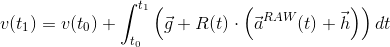
Forward speed

It would seem that much simpler. From school physics we know by definition

$\ vec {v} (t_1) = \ vec {v} (t_0) + \ int_ {t_0} ^ {t_1} \ vec {a} (t) dt$

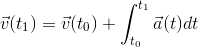
But we need speed in a fixed coordinate system, and the coordinate system of the accelerometer rotates with the device. Denote by R the rotation matrix from the device’s coordinate system to the fixed one, then

$\ vec {v} (t_1) = \ vec {v} (t_0) + \ int_ {t_0} ^ {t_1} R (t) \ vec {a} _ {D} (t) dt$

Where $\ vec {a} _ {D}$ - acceleration along the coordinate axes of the device. In turn, the rotation matrix is obtained simply by integrating the rotations measured by the gyroscope ( - derivative of the rotation matrix, it can be calculated, knowing the angular velocity around three axes):

$R (t_1) = R (t_0) + \ int_ {t_0} ^ {t_1} (I + W (t)) d t$

And everything? This was not the case, it works only for a spherical accelerometer in a vacuum. Let's look at the real data from the smartphone, lying motionless on the table:

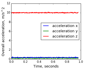
Raw accelerometer readings per axis

Observations:

The force of gravity is not automatically deducted, because the accelerometer cannot fundamentally distinguish the effect of the attraction of the earth from the effect of the acceleration of the phone. So you need to manually determine the direction and make an amendment. Theoretically, the android offers such an amendment at the OS level , but in practice it didn't really work for me.
The total acceleration / attraction along three axes passes over 10 m / s ² , which is very far from the tabular 9.81 m / s ² - in 10 minutes it will roll 0.2 * 600 = 120 m / s = 432 km / h.

The second experiment is to write the total acceleration from the phone lying on the table with the screen up, and then with the screen down, and compare:

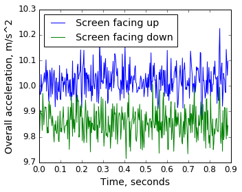
Overall measured acceleration up and down comparison

Observations:

The difference in excess of 0.15 m / s ^{2 is} simply a change in orientation, that is, there is a noticeable systematic error in the local coordinate system.
Constant noise measurements in the region of 0.05 m / s ² , and as we see from the integrals above - errors accumulate over time. And when the noises are summed up, then even with unbiased noise (i.e., when the expectation of the measurement coincides with the true value), according to the central limit theorem, the variance of the sum of n measurements will be $O \ left (\ sqrt {n} \ right)$ .

Model noise and auto calibration

So, to get a real acceleration in a fixed coordinate system, corrections to the "raw" measurements of the accelerometer are necessary. Let's apply a simple model:

$v (t_1) = v (t_0) + \ int_ {t_0} ^ {t_1} \ left (\ vec {g} + R (t) \ cdot \ left (\ vec {a} ^ {RAW} (t) + \ vec {h} \ right) \ right) dt$

Where

$\ vec {a} ^ {RAW}$ - raw accelerometer measurement, in the device coordinate system.
$\ vec {h}$ - compensation of the accelerometer systematic error, also in the device coordinate system.
- rotation matrix from the device coordinate system to the fixed coordinate system.
$\ vec {g}$ - constant force of the in the fixed coordinate system.

The rotation matrix will be obtained by integrating the angular velocities from the gyroscope, but the remaining parameters are unknown (including $\ vec {g}$ because unknown initial orientation of the smartphone). Find the calibration parameters with GPS data. Recall that GPS measurements are pretty accurate. So the speed calculated by inertial sensors should be close to the speed according to GPS . We formalize this intuition as an optimization problem. For each interval between adjacent GPS measurements (about 1 second), we calculate the distance traveled according to inertial data, and according to GPS data, and assign the target function to the L2 metric over the entire recording time:

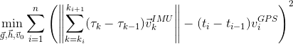
$\ min _ {\ vec {g}, \ vec {h}, \ vec {v} _0} \ sum_ {i = 1} ^ n \ left (\ left \ | \ sum_ {k = k_i} ^ {k_ {i +1}} (\ tau_k - \ tau_ {k-1}) \ vec {v} _k ^ {IMU} \ right \ | - (t_i - t_ {i-1}) v ^ {GPS} _i \ right) ^ 2$

Where

- GPS measurement index.
$k_i \ dots k_ {i + 1}$ - indices of measurement of inertial sensors that fall into the gap between measurements GPS i and i+1 .
$\ tau_j$ time measurement of inertial sensors.

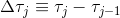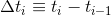Also denote $\ Delta \ tau_j \ equiv \ tau_j - \ tau_ {j-1}$ and $\ Delta t_i \ equiv t_i - t_ {i-1}$ , and substituting corrections to the raw measurements of the accelerometer, we obtain the final form of the objective function:

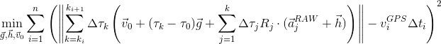
$\ min _ {\ vec {g}, \ vec {h}, \ vec {v} _0} \ sum_ {i = 1} ^ n \ left (\ left \ | \ sum_ {k = k_i} ^ {k_ {i +1}} \ Delta \ tau_k \ left (\ vec {v} _0 + (\ tau_k - \ tau_0) \ vec {g} + \ sum_ {j = 1} ^ k \ Delta \ tau_j R_j \ cdot (\ vec {a} _j ^ {RAW} + \ vec {h}) \ right) \ right \ | - v ^ {GPS} _i \ Delta t_i \ right) ^ 2$

It looks scary, but in fact it is a simple quadratic function, it is easy to take derivatives analytically and optimize using any numerical method, for example L-BFGS .

For a start, check on a short segment in half a minute:

calibration calibrated

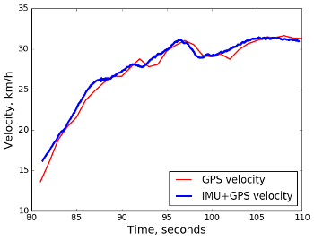
Here, “by eye” it is not very clear which graph is more correct, but it is possible to declare success, at least in the sense that it was possible to select calibration parameters of the amendments, with which the velocity estimates from two different sources are very close. Now let's try the same approach on a longer recording, about 10 minutes:

Something went wrong

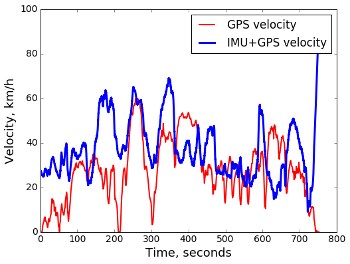
Here of course a complete failure. It turns out that the model of simple corrections is insufficient for long time intervals, that is, there are important sources of distortions that it does not take into account. It can be

Systematic errors ("care") of the gyroscope.
Accelerometer and gyroscope white noise accumulated over time $O (\ sqrt {t})$ by the central limit theorem .
Interaction with the engine vibrations (through the car body) when driving.

Local auto calibration by sliding window

To deal with the problems of a simple model of amendments for inertial sensors can be different. Possible options:

Improve accuracy by simulating unaccounted sources of error (gyroscope drift, white noise accumulation).
Cheat

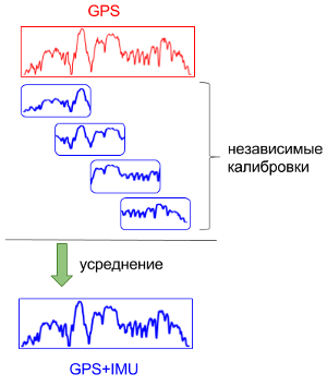
We cheat. After all, in the end, we are not interested in the calibration model itself, but in the final speed values. And if the calibration copes on short segments, you can use the standard technique with a sliding window:

we divide the full time interval into overlapping short segments,
on each segment, separately, we calibrate and calculate the speed by integration,
we average the result for each point in time over the segments that include it:

sliding window

Final result:

Final result - long-range time series calibrated with overlapping sliding windows

We declare success with a forward speed, we return to the angular speed of turns.

Corner speed

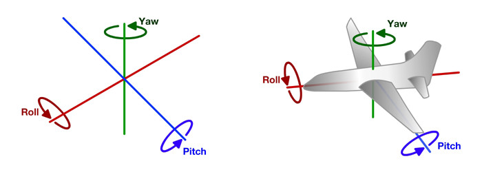
The angular speed of rotation is needed to calculate the radius of rotation (and, accordingly, the angle of rotation of the steering wheel): $r = v / \ omega$ . The gyroscope measures the angular velocity directly, but in three-dimensional space: in addition to the rotation around the vertical axis (yaw - actually turns), the data also reflects rotation around the transverse (pitch - change of the road gradient, passage of speed bumps) and longitudinal (roll - ride one side in a rut or pit):

pitch-roll-yaw

We need to select from the three-dimensional rotations only the component around the vertical axis (in the coordinate system of the car). Accordingly, you need to get the direction of this axis. To do this, we use the observation that the magnitude of rotation around the vertical axis is much larger than around the longitudinal and transverse (turns at 90 degrees is the norm, but fortunately, there is no change of slope and track). So you can simply take the axis around which the total rotation was maximum, for the vertical.

Mathematically, it is convenient to isolate the dominant rotation axis by presenting each elementary rotation (that is, measuring a gyroscope) in the form of a quaternion. Rotation around the unit axis (x,y,z) at an angle $\ theta$ seems to be a quaternion

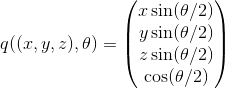
$q ((x, y, z), \ theta) = \ begin {pmatrix} x \ sin (\ theta / 2) \\ y \ sin (\ theta / 2) \\ z \ sin (\ theta / 2) \\ cos (\ theta / 2) \ end {pmatrix}$

The convenience is that the first three components of the quaternion characterize simultaneously the direction of the axis of rotation and the amount of rotation. Therefore, a good result is provided by the principal component method applied simply to the first three components of the quaternion. After selecting the dominant axis, it turns out this picture:

Rotations after PCA

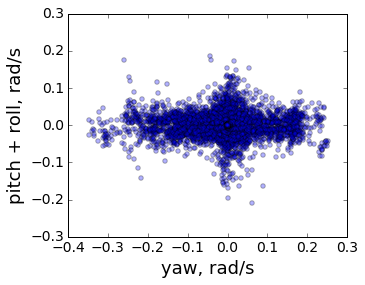
It can be seen that a noticeably larger proportion of rotations passes around the selected dominant axis than around the other two perpendicular to it.

By the way, in the previous post , the principal component method was also applied, but then I did not realize to apply it to rotations directly, but selected a horizontal plane along a three-dimensional trajectory (that is, based on displacements instead of rotations). The new method is better not only because it does not completely need information about the displacements, but also because the vertical axis stands out in the coordinate system of the device . That is, with the new approach, the vertical axis is perpendicular to the local plane of the road, instead of the median plane of the entire trajectory in the old approach. For example, now the vertical axis turns (together with the car when moving from the road uphill to the road downhill). As a result, the selection of the horizontal rotation of the total rotation has become more accurate.

Data

Bonus to the code I want to share the already processed data for those who are interested to play with the training of their models. In the torrent there are more than an hour of raw data recorded on the roads near Moscow, plus (in postprocessed directories) the results of calculating the translational speed and the angular speed of turns. If you use - it will be interesting to know about the results!

That's all, in the next series - learn how to predict the control actions from video.

Source: https://habr.com/ru/post/329484/

All Articles