Evaluation of the quality of face recognition algorithms
Hi, Habr!
At NtechLab, we are engaged in research and development of face recognition products. In the process of implementing our solutions, we often encounter the fact that customers are not very clear about the requirements for the accuracy of the algorithm, so testing one solution or another for their task is difficult. To remedy the situation, we developed a brief guide describing the main metrics and testing approaches, which I would like to share with the Habr community.
')
In recent times, facial recognition is gaining more and more interest from the commercial sector and the state. However, the correct measurement of the accuracy of such systems is not an easy task and contains a lot of nuances. We are constantly being asked to test our technology and pilot projects based on it, and we noticed that there are often questions about the terminology and methods of testing algorithms for business problems. As a result, inappropriate tools may be selected to solve the problem, resulting in financial losses or lost profits. We decided to publish this note to help people master the environment of specialized terms and raw data surrounding face recognition technology. We wanted to talk about the basic concepts in this area in a simple and understandable language. Hopefully, this will allow technical and entrepreneurial people to speak the same language, better understand the scenarios of using face recognition in the real world and make decisions confirmed by data.
Face recognition is often called a set of different tasks, such as detecting a person in a photo or in a video stream, determining gender and age, searching for the right person among multiple images, or checking that the same person is in two images. In this article we will focus on the last two tasks and we will call them, respectively, identification and verification. To solve these problems, special descriptors or feature vectors are extracted from images. In this case, the task of identification is reduced to finding the nearest feature vector, and verification can be implemented using a simple threshold of distances between the vectors. By combining these two actions, you can identify a person among a set of images or decide that he is not among those images. Such a procedure is called open-set identification (see identification on an open set), see Fig.1.

Fig.1 Open-set identification
For a quantitative assessment of the similarity of persons, you can use the distance in the space of feature vectors. Often choose Euclidean or cosine distance, but there are other, more complex, approaches. The specific distance function is often supplied as part of a face recognition product. Identification and verification return different results and, accordingly, different metrics are used to assess their quality. We will look at quality metrics in detail in the following sections. In addition to choosing an adequate metric, to assess the accuracy of the algorithm, you will need a marked set of images (datasets).
Almost all modern facial recognition software is built on machine learning. Algorithms are trained in large datasets (datasets) with tagged images. Both the quality and nature of these datasets have a significant impact on accuracy. The better the source data, the better the algorithm will cope with the task.
A natural way to verify that the accuracy of the face recognition algorithm meets expectations is to measure the accuracy on a separate test dataset. It is very important to choose this dataset correctly. In the ideal case, the organization should acquire its own set of data as closely as possible with the images with which the system will work during operation. Pay attention to the camera, shooting conditions, age, gender and nationality of people who fall into the test dataset. The more similar the test data to the real data, the more reliable the test results will be. Therefore, it often makes sense to spend time and money collecting and marking your data set. If this is not possible for some reason, you can use public datasets, for example, LFW and MegaFace . LFW contains only 6000 pairs of face images and is not suitable for many real-life scenarios: in particular, it’s impossible to measure low enough error levels on this dataset, as we will see later. Dataset MegaFace contains much more images and is suitable for testing face recognition algorithms on a large scale. However, the MegaFace training and test set of images is publicly available, so it should be used for testing with caution.
An alternative is to use the test results by a third party. Such tests are conducted by qualified specialists on large closed datasets, and their results can be trusted. One example is the NIST Face Recognition Vendor Test Ongoing . This is a test conducted by the National Institute of Standards and Technology (NIST) at the US Department of Commerce. The “minus” of this approach is that the data of the testing organization may differ significantly from the use case of interest.
As we said, machine learning is at the core of modern facial recognition software. One of the common phenomena of machine learning is the so-called. retraining. It manifests itself in the fact that the algorithm shows good results on the data used in the training, but the results on the new data are much worse.
Consider a specific example: imagine a client who wants to establish a bandwidth system with face recognition. For these purposes, he collects a set of photos of people who will be allowed access, and teaches the algorithm to distinguish them from other people. On tests, the system shows good results and is being put into operation. After some time, the list of people with admission decide to expand and it turns out that the system denies new people access. The algorithm was tested on the same data as it was trained, and no one measured the accuracy on new photos. This, of course, is an exaggerated example, but it allows you to understand the problem.
In some cases, retraining is not so obvious. Suppose the algorithm was trained on the images of people, where a certain ethnic group prevailed. When applying such an algorithm to persons of other nationalities, its accuracy will certainly fall. An overly optimistic assessment of the accuracy of the algorithm due to incorrect testing is a very common mistake. You should always test the algorithm on new data that it has to process in real application, and not on the data on which the training was conducted.
Summarizing the above, we make a list of recommendations: do not use the data on which the algorithm has been trained for testing, use a special closed dataset for testing. If this is not possible and you are going to use a public dataset, make sure that the vendor has not used it in the process of learning and / or setting up the algorithm. Learn datasets before testing, consider how close it is to the data that will come from operating the system.
After selecting the dataset, you should decide on the metric that will be used to evaluate the results. In general, a metric is a function that accepts the input of the results of the algorithm (identification or verification), and returns a number that corresponds to the quality of the algorithm on a particular dataset. Using the same number for a quantitative comparison of different algorithms or vendors allows for a succinct presentation of test results and facilitates the decision-making process. In this section, we will look at the metrics most commonly used in face recognition, and discuss their meaning from a business perspective.
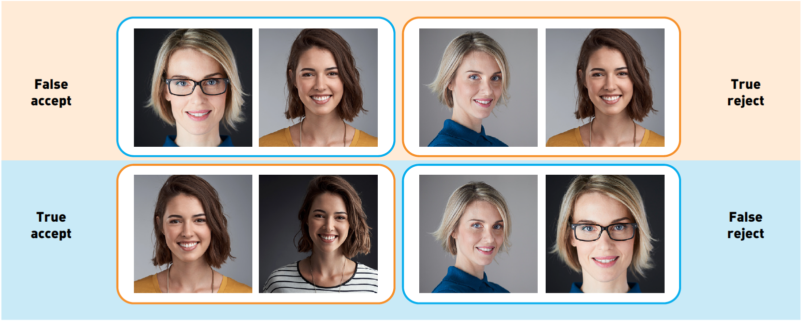
Verification of individuals can be viewed as a binary decision making process: “yes” (two images belong to the same person), “no” (different people are depicted on a pair of photos). Before dealing with verification metrics, it is helpful to understand how we can classify errors in such problems. Given that there are 2 possible responses of the algorithm and 2 variants of the true state of affairs, there are only 4 possible outcomes:
Fig. 2 Types of errors. The background color encodes the true relationship between the pictures (blue means “accept”, yellow - “reject”), the color of the frame corresponds to the prediction of the algorithm (blue - “accept”, yellow - “reject”

In the table above, the columns correspond to the solution of the algorithm (blue to accept, yellow to reject), the lines correspond to the true values (encoded in the same colors). The correct answers of the algorithm are marked with a green background, erroneous - with red.
Of these outcomes, two correspond to the correct answers of the algorithm, and two correspond to errors of the first and second kind, respectively. Errors of the first kind are called “false accept”, “false positive” or “false match” (incorrectly accepted), and errors of the second kind - “false reject”, “false negative” or “false non-match” (incorrectly rejected).
Summing up the number of errors of various kinds among pairs of images in dataset and dividing them by the number of pairs, we get the false accept rate (FAR) and false reject rate (FRR). In the case of an access control system, “false positive” corresponds to giving access to a person for whom this access is not provided, while “false negative” means that the system mistakenly denied access to an authorized person. These errors have different costs in terms of business and are therefore considered separately. In the access control example, “false negative” causes the security officer to recheck the employee's pass. Providing unauthorized access to a potential violator (false positive) can lead to much worse consequences.
Given that various types of errors are associated with various risks, manufacturers of face recognition software often provide the opportunity to customize the algorithm so as to minimize one type of error. For this, the algorithm returns not a binary value, but a real number, which reflects the confidence of the algorithm in its decision. In this case, the user can independently select the threshold and fix the level of errors at certain values.
For example, consider the “toy” dataset of three images. Let images 1 and 2 belong to the same person, and image 3 to someone else. Suppose that the program assessed its confidence for each of the three pairs as follows:
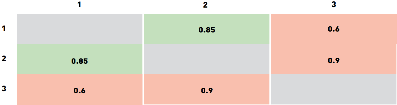
We specifically chose values in such a way that no threshold would classify all three pairs correctly. In particular, any threshold below 0.6 will result in two false accept (for pairs 2-3 and 1-3). Of course, this result can be improved.
Choosing a threshold from the range of 0.6 to 0.85 will result in a pair of 1-3 being rejected, a pair of 1-2 will still be accepted, and 2-3 will be falsely accepted. If you increase the threshold to 0.85-0.9, then a pair of 1-2 will be falsely rejected. Threshold values above 0.9 will result in two true rejects (pairs 1-3 and 2-3) and one false reject (1-2). Thus, the best options are thresholds from the range of 0.6-0.85 (one false accept 2-3) and a threshold above 0.9 (results in false reject 1-2). What value to choose as the final depends on the cost of errors of different types. In this example, the threshold varies over wide ranges, this is primarily due to the very small size of the data and to how we chose the confidence values of the algorithm. For large datasets used for real-life tasks, we would have significantly more accurate threshold values. Often, face recognition software vendors supply default threshold values for different FARs that are calculated in a similar way on the vendor's own datasets.
It is also easy to see that as the FAR of interest decreases, more and more positive pairs of images are required to accurately calculate the threshold value. So, for FAR = 0.001 you need at least 1000 pairs, and for FAR = It will take 1 million pairs. It is not easy to collect and mark up such data, so for customers interested in low FAR values, it makes sense to pay attention to public benchmarks, such as NIST Face Recognition Vendor Test or MegaFace . The latter should be treated with caution, since both the training and the test sample are available to everyone, which can lead to an overly optimistic assessment of accuracy (see the “Retraining” section).
Types of errors differ in their associated cost, and the client has a way to shift the balance towards those or other errors. For this we need to consider a wide range of threshold values. A convenient way to visualize the accuracy of the algorithm for different values of FAR is to build ROC curves (receiver operating characteristic, receiver operating characteristics).
Let's understand how ROC curves are constructed and analyzed. The confidence of the algorithm (and, consequently, the threshold) take values from a fixed interval. In other words, these quantities are bounded above and below. Suppose that this is an interval from 0 to 1. Now we can measure the number of errors by varying the threshold value from 0 to 1 in small steps. So, for each threshold value we get the FAR and TAR values (true accept rate). Next, we will draw each point so that FAR corresponds to the abscissa axis, and TAR corresponds to the ordinate axis.

Fig.3 Example of a ROC curve
It is easy to see that the first point will have coordinates of 1.1. With a threshold of 0, we accept all pairs and do not reject any. Similarly, the last point will be 0.0: at threshold 1, we do not accept a single pair and reject all pairs. At the other points, the curve is usually convex. You can also notice that the worst curve lies approximately on the diagonal of the graph and corresponds to a random guessing of the outcome. On the other hand, the best possible curve forms a triangle with vertices (0,0) (0,1) and (1,1). But on datasets of reasonable size it is difficult to meet.

Fig.4 NIST FRVT ROC curves
It is possible to construct a similarity of ROC curves with different metrics / errors on the axis. Consider, for example, Figure 4. It shows that the organizers of NIST FRVT on the Y axis painted FRR (in the picture - False non-match rate), and on the X axis - FAR (in the picture - False match rate). In this particular case, the best results are achieved by curves that are located below and shifted to the left, which corresponds to low FRR and FAR. Therefore, it is worth paying attention to what values are plotted along the axes.
Such a graph makes it easy to judge the accuracy of the algorithm for a given FAR: it suffices to find a point on a curve with a coordinate X equal to the desired FAR and the corresponding TAR value. The “quality” of a ROC curve can also be estimated by a single number, for this it is necessary to calculate the area under it. In this case, the best possible value will be 1, and a value of 0.5 corresponds to a random guessing. This number is called ROC AUC (Area Under Curve). However, it should be noted that the ROC AUC implicitly assumes that errors of the first and second kind are unambiguous, which is not always the case. If the price of errors varies, you should pay attention to the shape of the curve and the areas where FAR meets business requirements.
The second popular task of face recognition is the identification, or search for a person among a set of images. Search results are sorted according to the confidence of the algorithm, and the most likely matches fall to the top of the list. Depending on whether or not the desired person is present in the search base, identification is divided into two subcategories: closed-set identification (it is known that the desired person is in the database) and open-set identification (the desired person may not be in the database).
Accuracy (accuracy) is a reliable and understandable metric for closed-set identification. In fact, accuracy measures the number of times that a person has been among the search results.
How does it work in practice? Let's figure it out. Let's start with the business requirements statement. Suppose we have a web page that can host ten search results. We need to measure the number of times that the desired person falls into the first ten responses of the algorithm. This number is called Top-N accuracy (in this particular case, N is 10).
For each test, we define the image of the person we are looking for and the gallery in which we search, so that the gallery contains at least one more image of this person. We review the first ten results of the search algorithm and check if there is a person among them. To obtain accuracy, one should sum up all the tests in which the desired person was in the search results, and divide by the total number of tests.

Figure 5. An example of identification. In this example, the desired person appears at position 2, so the accuracy of Top-1 is 0, and Top-2 and later is 1.
Open-set identification consists of finding people who are most similar to the desired image, and determining whether one of them is the desired person based on the confidence of the algorithm. Open-set identification can be viewed as a combination of closed-set identification and verification, so all the same metrics can be used for this task as in the verification task. It is also easy to see that the open-set identification can be reduced to pair-wise comparisons of the desired image with all the images from the gallery. In practice, this is not used for speed considerations. Facial recognition software often comes with fast search algorithms that can find among millions of people alike in milliseconds. Pairwise comparisons would take much longer.
As an illustration, let's look at a few common situations and approaches to testing face recognition algorithms.
Suppose that an average-sized retail store wants to improve its loyalty program or reduce the number of thefts. It's funny, but from the point of view of face recognition, this is about the same thing. The main task of this project is to identify the customer or the attacker as early as possible from the camera image and pass this information on to the seller or security officer.
Let loyalty program encompass 100 clients. This task can be considered as an example of open-set identification. Assessing the costs, the marketing department concluded that the acceptable level of error was to take one visitor as a regular customer per day. If a day is visited by 1000 visitors, each of which must be checked with a list of 100 regular customers, then the required FAR will be .
Having determined the acceptable error level, you should select the appropriate dataset for testing. A good option would be to place the camera in a suitable place (vendors can help with a specific device and location). By comparing the transactions of the regular customers with the images from the camera and having carried out manual filtering, store employees can collect a set of positive pairs. It also makes sense to collect a set of images of random visitors (one image per person). The total number of images should roughly correspond to the number of visitors to the store per day. By combining both sets, you can get datasets of both “positive” and “negative” pairs.
To test the desired accuracy should be enough for about a thousand "positive" pairs. By combining various regular customers and occasional visitors, you can collect about 100,000 "negative" pairs.
The next step will be to run (or ask the vendor to run) the software and get the confidence of the algorithm for each pair from the dataset. When this is done, you can build a ROC curve and make sure that the number of correctly identified regular customers with FAR = Meets business requirements.
Modern airports serve tens of millions of passengers a year, and about 300,000 people pass through the passport control procedure every day. Automation of this process will significantly reduce costs. On the other hand, it is highly undesirable to miss the intruder, and the airport administration wants to minimize the risk of such an event. FAR = corresponds to ten violators per year and seems reasonable in this situation. If with this FAR, FRR is 0.1 (which corresponds to the NtechLab results on the NIST visa images benchmark), then the cost of manual verification of documents can be reduced tenfold. However, in order to assess the accuracy at a given level of FAR, tens of millions of images will be needed. The collection of such a large dataset requires significant funds and may require additional coordination of the processing of personal data. As a result, investment in such a system can pay off for too long. In this case, it makes sense to refer to the NIST Face Recognition Vendor Test test report, which contains datasets with photos of visas. The airport administration should choose a vendor based on testing on this dataset, taking into account the passenger traffic.
So far, we have considered examples in which the customer was interested in low FAR, but this is not always the case. Imagine a camera-equipped stand in a large shopping center. The shopping center has its own loyalty program and would like to identify its participants who stopped at the booth. Further, these buyers could be sent targeted letters with discounts and interesting offers on the basis that they were interested on the stand.
Suppose that the operation of such a system costs $ 10, while about 1000 visitors a day stop at the stand. The marketing department estimated the profit from each targeted email at $ 0.0105. We would like to identify as many loyal customers as possible and not disturb others too much. For such a distribution to pay off, the accuracy must be equal to the cost of the stand, divided by the number of visitors and the expected income from each letter. For our example, the accuracy is . The mall administration could collect the data in the manner described in the “Retail Store” section and measure the accuracy as described in the “Identification” section. Based on the test results, you can decide whether to get the expected benefits using the face recognition system.
In this article we discussed mainly the work with images and almost did not deal with streaming video.Video can be viewed as a sequence of static images, so the metrics and approaches to testing accuracy on images are applicable to video. It should be noted that the processing of streaming video is much more costly in terms of the calculations and imposes additional restrictions on all stages of face recognition. When working with video, separate performance testing should be carried out, so the details of this process are not covered in this text.
In this section, we would like to list common problems and errors encountered when testing facial recognition software and give recommendations on how to avoid them.
. . , FAR/TAR. «» «» , , . .
Sometimes people test a face recognition algorithm with one fixed threshold (often chosen by the manufacturer as “default”) and take into account only one type of error. This is wrong, since the default threshold values for different vendors are different or are selected based on different FAR or TAR values. When testing, you should pay attention to both types of errors.
Datasets vary in size, quality and complexity, so the results of the algorithms on different datasets cannot be compared. You can easily refuse the best solution just because it was tested on a more complex than a competitor dataset.
You should try to test on multiple data sets. When choosing a single public dataset, one cannot be sure that it was not used when training or setting up an algorithm. In this case, the accuracy of the algorithm will be overestimated. Fortunately, the probability of this event can be reduced by comparing the results on different datasets.
: , , .
, , , ( NtechLab ). , , -.
At NtechLab, we are engaged in research and development of face recognition products. In the process of implementing our solutions, we often encounter the fact that customers are not very clear about the requirements for the accuracy of the algorithm, so testing one solution or another for their task is difficult. To remedy the situation, we developed a brief guide describing the main metrics and testing approaches, which I would like to share with the Habr community.
')
In recent times, facial recognition is gaining more and more interest from the commercial sector and the state. However, the correct measurement of the accuracy of such systems is not an easy task and contains a lot of nuances. We are constantly being asked to test our technology and pilot projects based on it, and we noticed that there are often questions about the terminology and methods of testing algorithms for business problems. As a result, inappropriate tools may be selected to solve the problem, resulting in financial losses or lost profits. We decided to publish this note to help people master the environment of specialized terms and raw data surrounding face recognition technology. We wanted to talk about the basic concepts in this area in a simple and understandable language. Hopefully, this will allow technical and entrepreneurial people to speak the same language, better understand the scenarios of using face recognition in the real world and make decisions confirmed by data.
Face recognition tasks
Face recognition is often called a set of different tasks, such as detecting a person in a photo or in a video stream, determining gender and age, searching for the right person among multiple images, or checking that the same person is in two images. In this article we will focus on the last two tasks and we will call them, respectively, identification and verification. To solve these problems, special descriptors or feature vectors are extracted from images. In this case, the task of identification is reduced to finding the nearest feature vector, and verification can be implemented using a simple threshold of distances between the vectors. By combining these two actions, you can identify a person among a set of images or decide that he is not among those images. Such a procedure is called open-set identification (see identification on an open set), see Fig.1.
Fig.1 Open-set identification
For a quantitative assessment of the similarity of persons, you can use the distance in the space of feature vectors. Often choose Euclidean or cosine distance, but there are other, more complex, approaches. The specific distance function is often supplied as part of a face recognition product. Identification and verification return different results and, accordingly, different metrics are used to assess their quality. We will look at quality metrics in detail in the following sections. In addition to choosing an adequate metric, to assess the accuracy of the algorithm, you will need a marked set of images (datasets).
Accuracy Assessment
Datasets
Almost all modern facial recognition software is built on machine learning. Algorithms are trained in large datasets (datasets) with tagged images. Both the quality and nature of these datasets have a significant impact on accuracy. The better the source data, the better the algorithm will cope with the task.
A natural way to verify that the accuracy of the face recognition algorithm meets expectations is to measure the accuracy on a separate test dataset. It is very important to choose this dataset correctly. In the ideal case, the organization should acquire its own set of data as closely as possible with the images with which the system will work during operation. Pay attention to the camera, shooting conditions, age, gender and nationality of people who fall into the test dataset. The more similar the test data to the real data, the more reliable the test results will be. Therefore, it often makes sense to spend time and money collecting and marking your data set. If this is not possible for some reason, you can use public datasets, for example, LFW and MegaFace . LFW contains only 6000 pairs of face images and is not suitable for many real-life scenarios: in particular, it’s impossible to measure low enough error levels on this dataset, as we will see later. Dataset MegaFace contains much more images and is suitable for testing face recognition algorithms on a large scale. However, the MegaFace training and test set of images is publicly available, so it should be used for testing with caution.
An alternative is to use the test results by a third party. Such tests are conducted by qualified specialists on large closed datasets, and their results can be trusted. One example is the NIST Face Recognition Vendor Test Ongoing . This is a test conducted by the National Institute of Standards and Technology (NIST) at the US Department of Commerce. The “minus” of this approach is that the data of the testing organization may differ significantly from the use case of interest.
Retraining
As we said, machine learning is at the core of modern facial recognition software. One of the common phenomena of machine learning is the so-called. retraining. It manifests itself in the fact that the algorithm shows good results on the data used in the training, but the results on the new data are much worse.
Consider a specific example: imagine a client who wants to establish a bandwidth system with face recognition. For these purposes, he collects a set of photos of people who will be allowed access, and teaches the algorithm to distinguish them from other people. On tests, the system shows good results and is being put into operation. After some time, the list of people with admission decide to expand and it turns out that the system denies new people access. The algorithm was tested on the same data as it was trained, and no one measured the accuracy on new photos. This, of course, is an exaggerated example, but it allows you to understand the problem.
In some cases, retraining is not so obvious. Suppose the algorithm was trained on the images of people, where a certain ethnic group prevailed. When applying such an algorithm to persons of other nationalities, its accuracy will certainly fall. An overly optimistic assessment of the accuracy of the algorithm due to incorrect testing is a very common mistake. You should always test the algorithm on new data that it has to process in real application, and not on the data on which the training was conducted.
Summarizing the above, we make a list of recommendations: do not use the data on which the algorithm has been trained for testing, use a special closed dataset for testing. If this is not possible and you are going to use a public dataset, make sure that the vendor has not used it in the process of learning and / or setting up the algorithm. Learn datasets before testing, consider how close it is to the data that will come from operating the system.
Metrics
After selecting the dataset, you should decide on the metric that will be used to evaluate the results. In general, a metric is a function that accepts the input of the results of the algorithm (identification or verification), and returns a number that corresponds to the quality of the algorithm on a particular dataset. Using the same number for a quantitative comparison of different algorithms or vendors allows for a succinct presentation of test results and facilitates the decision-making process. In this section, we will look at the metrics most commonly used in face recognition, and discuss their meaning from a business perspective.
Verification
Verification of individuals can be viewed as a binary decision making process: “yes” (two images belong to the same person), “no” (different people are depicted on a pair of photos). Before dealing with verification metrics, it is helpful to understand how we can classify errors in such problems. Given that there are 2 possible responses of the algorithm and 2 variants of the true state of affairs, there are only 4 possible outcomes:
Fig. 2 Types of errors. The background color encodes the true relationship between the pictures (blue means “accept”, yellow - “reject”), the color of the frame corresponds to the prediction of the algorithm (blue - “accept”, yellow - “reject”
In the table above, the columns correspond to the solution of the algorithm (blue to accept, yellow to reject), the lines correspond to the true values (encoded in the same colors). The correct answers of the algorithm are marked with a green background, erroneous - with red.
Of these outcomes, two correspond to the correct answers of the algorithm, and two correspond to errors of the first and second kind, respectively. Errors of the first kind are called “false accept”, “false positive” or “false match” (incorrectly accepted), and errors of the second kind - “false reject”, “false negative” or “false non-match” (incorrectly rejected).
Summing up the number of errors of various kinds among pairs of images in dataset and dividing them by the number of pairs, we get the false accept rate (FAR) and false reject rate (FRR). In the case of an access control system, “false positive” corresponds to giving access to a person for whom this access is not provided, while “false negative” means that the system mistakenly denied access to an authorized person. These errors have different costs in terms of business and are therefore considered separately. In the access control example, “false negative” causes the security officer to recheck the employee's pass. Providing unauthorized access to a potential violator (false positive) can lead to much worse consequences.
Given that various types of errors are associated with various risks, manufacturers of face recognition software often provide the opportunity to customize the algorithm so as to minimize one type of error. For this, the algorithm returns not a binary value, but a real number, which reflects the confidence of the algorithm in its decision. In this case, the user can independently select the threshold and fix the level of errors at certain values.
For example, consider the “toy” dataset of three images. Let images 1 and 2 belong to the same person, and image 3 to someone else. Suppose that the program assessed its confidence for each of the three pairs as follows:
We specifically chose values in such a way that no threshold would classify all three pairs correctly. In particular, any threshold below 0.6 will result in two false accept (for pairs 2-3 and 1-3). Of course, this result can be improved.
Choosing a threshold from the range of 0.6 to 0.85 will result in a pair of 1-3 being rejected, a pair of 1-2 will still be accepted, and 2-3 will be falsely accepted. If you increase the threshold to 0.85-0.9, then a pair of 1-2 will be falsely rejected. Threshold values above 0.9 will result in two true rejects (pairs 1-3 and 2-3) and one false reject (1-2). Thus, the best options are thresholds from the range of 0.6-0.85 (one false accept 2-3) and a threshold above 0.9 (results in false reject 1-2). What value to choose as the final depends on the cost of errors of different types. In this example, the threshold varies over wide ranges, this is primarily due to the very small size of the data and to how we chose the confidence values of the algorithm. For large datasets used for real-life tasks, we would have significantly more accurate threshold values. Often, face recognition software vendors supply default threshold values for different FARs that are calculated in a similar way on the vendor's own datasets.
It is also easy to see that as the FAR of interest decreases, more and more positive pairs of images are required to accurately calculate the threshold value. So, for FAR = 0.001 you need at least 1000 pairs, and for FAR = It will take 1 million pairs. It is not easy to collect and mark up such data, so for customers interested in low FAR values, it makes sense to pay attention to public benchmarks, such as NIST Face Recognition Vendor Test or MegaFace . The latter should be treated with caution, since both the training and the test sample are available to everyone, which can lead to an overly optimistic assessment of accuracy (see the “Retraining” section).
Types of errors differ in their associated cost, and the client has a way to shift the balance towards those or other errors. For this we need to consider a wide range of threshold values. A convenient way to visualize the accuracy of the algorithm for different values of FAR is to build ROC curves (receiver operating characteristic, receiver operating characteristics).
Let's understand how ROC curves are constructed and analyzed. The confidence of the algorithm (and, consequently, the threshold) take values from a fixed interval. In other words, these quantities are bounded above and below. Suppose that this is an interval from 0 to 1. Now we can measure the number of errors by varying the threshold value from 0 to 1 in small steps. So, for each threshold value we get the FAR and TAR values (true accept rate). Next, we will draw each point so that FAR corresponds to the abscissa axis, and TAR corresponds to the ordinate axis.
Fig.3 Example of a ROC curve
It is easy to see that the first point will have coordinates of 1.1. With a threshold of 0, we accept all pairs and do not reject any. Similarly, the last point will be 0.0: at threshold 1, we do not accept a single pair and reject all pairs. At the other points, the curve is usually convex. You can also notice that the worst curve lies approximately on the diagonal of the graph and corresponds to a random guessing of the outcome. On the other hand, the best possible curve forms a triangle with vertices (0,0) (0,1) and (1,1). But on datasets of reasonable size it is difficult to meet.
Fig.4 NIST FRVT ROC curves
It is possible to construct a similarity of ROC curves with different metrics / errors on the axis. Consider, for example, Figure 4. It shows that the organizers of NIST FRVT on the Y axis painted FRR (in the picture - False non-match rate), and on the X axis - FAR (in the picture - False match rate). In this particular case, the best results are achieved by curves that are located below and shifted to the left, which corresponds to low FRR and FAR. Therefore, it is worth paying attention to what values are plotted along the axes.
Such a graph makes it easy to judge the accuracy of the algorithm for a given FAR: it suffices to find a point on a curve with a coordinate X equal to the desired FAR and the corresponding TAR value. The “quality” of a ROC curve can also be estimated by a single number, for this it is necessary to calculate the area under it. In this case, the best possible value will be 1, and a value of 0.5 corresponds to a random guessing. This number is called ROC AUC (Area Under Curve). However, it should be noted that the ROC AUC implicitly assumes that errors of the first and second kind are unambiguous, which is not always the case. If the price of errors varies, you should pay attention to the shape of the curve and the areas where FAR meets business requirements.
Identification
The second popular task of face recognition is the identification, or search for a person among a set of images. Search results are sorted according to the confidence of the algorithm, and the most likely matches fall to the top of the list. Depending on whether or not the desired person is present in the search base, identification is divided into two subcategories: closed-set identification (it is known that the desired person is in the database) and open-set identification (the desired person may not be in the database).
Accuracy (accuracy) is a reliable and understandable metric for closed-set identification. In fact, accuracy measures the number of times that a person has been among the search results.
How does it work in practice? Let's figure it out. Let's start with the business requirements statement. Suppose we have a web page that can host ten search results. We need to measure the number of times that the desired person falls into the first ten responses of the algorithm. This number is called Top-N accuracy (in this particular case, N is 10).
For each test, we define the image of the person we are looking for and the gallery in which we search, so that the gallery contains at least one more image of this person. We review the first ten results of the search algorithm and check if there is a person among them. To obtain accuracy, one should sum up all the tests in which the desired person was in the search results, and divide by the total number of tests.
Figure 5. An example of identification. In this example, the desired person appears at position 2, so the accuracy of Top-1 is 0, and Top-2 and later is 1.
Open-set identification consists of finding people who are most similar to the desired image, and determining whether one of them is the desired person based on the confidence of the algorithm. Open-set identification can be viewed as a combination of closed-set identification and verification, so all the same metrics can be used for this task as in the verification task. It is also easy to see that the open-set identification can be reduced to pair-wise comparisons of the desired image with all the images from the gallery. In practice, this is not used for speed considerations. Facial recognition software often comes with fast search algorithms that can find among millions of people alike in milliseconds. Pairwise comparisons would take much longer.
Practical examples
As an illustration, let's look at a few common situations and approaches to testing face recognition algorithms.
Retail store
Suppose that an average-sized retail store wants to improve its loyalty program or reduce the number of thefts. It's funny, but from the point of view of face recognition, this is about the same thing. The main task of this project is to identify the customer or the attacker as early as possible from the camera image and pass this information on to the seller or security officer.
Let loyalty program encompass 100 clients. This task can be considered as an example of open-set identification. Assessing the costs, the marketing department concluded that the acceptable level of error was to take one visitor as a regular customer per day. If a day is visited by 1000 visitors, each of which must be checked with a list of 100 regular customers, then the required FAR will be .
Having determined the acceptable error level, you should select the appropriate dataset for testing. A good option would be to place the camera in a suitable place (vendors can help with a specific device and location). By comparing the transactions of the regular customers with the images from the camera and having carried out manual filtering, store employees can collect a set of positive pairs. It also makes sense to collect a set of images of random visitors (one image per person). The total number of images should roughly correspond to the number of visitors to the store per day. By combining both sets, you can get datasets of both “positive” and “negative” pairs.
To test the desired accuracy should be enough for about a thousand "positive" pairs. By combining various regular customers and occasional visitors, you can collect about 100,000 "negative" pairs.
The next step will be to run (or ask the vendor to run) the software and get the confidence of the algorithm for each pair from the dataset. When this is done, you can build a ROC curve and make sure that the number of correctly identified regular customers with FAR = Meets business requirements.
E-Gate at the airport
Modern airports serve tens of millions of passengers a year, and about 300,000 people pass through the passport control procedure every day. Automation of this process will significantly reduce costs. On the other hand, it is highly undesirable to miss the intruder, and the airport administration wants to minimize the risk of such an event. FAR = corresponds to ten violators per year and seems reasonable in this situation. If with this FAR, FRR is 0.1 (which corresponds to the NtechLab results on the NIST visa images benchmark), then the cost of manual verification of documents can be reduced tenfold. However, in order to assess the accuracy at a given level of FAR, tens of millions of images will be needed. The collection of such a large dataset requires significant funds and may require additional coordination of the processing of personal data. As a result, investment in such a system can pay off for too long. In this case, it makes sense to refer to the NIST Face Recognition Vendor Test test report, which contains datasets with photos of visas. The airport administration should choose a vendor based on testing on this dataset, taking into account the passenger traffic.
Targeted Mailing List
So far, we have considered examples in which the customer was interested in low FAR, but this is not always the case. Imagine a camera-equipped stand in a large shopping center. The shopping center has its own loyalty program and would like to identify its participants who stopped at the booth. Further, these buyers could be sent targeted letters with discounts and interesting offers on the basis that they were interested on the stand.
Suppose that the operation of such a system costs $ 10, while about 1000 visitors a day stop at the stand. The marketing department estimated the profit from each targeted email at $ 0.0105. We would like to identify as many loyal customers as possible and not disturb others too much. For such a distribution to pay off, the accuracy must be equal to the cost of the stand, divided by the number of visitors and the expected income from each letter. For our example, the accuracy is . The mall administration could collect the data in the manner described in the “Retail Store” section and measure the accuracy as described in the “Identification” section. Based on the test results, you can decide whether to get the expected benefits using the face recognition system.
Video support
In this article we discussed mainly the work with images and almost did not deal with streaming video.Video can be viewed as a sequence of static images, so the metrics and approaches to testing accuracy on images are applicable to video. It should be noted that the processing of streaming video is much more costly in terms of the calculations and imposes additional restrictions on all stages of face recognition. When working with video, separate performance testing should be carried out, so the details of this process are not covered in this text.
Common mistakes
In this section, we would like to list common problems and errors encountered when testing facial recognition software and give recommendations on how to avoid them.
Insufficient dataset testing
. . , FAR/TAR. «» «» , , . .
Sometimes people test a face recognition algorithm with one fixed threshold (often chosen by the manufacturer as “default”) and take into account only one type of error. This is wrong, since the default threshold values for different vendors are different or are selected based on different FAR or TAR values. When testing, you should pay attention to both types of errors.
Comparing results on different datasets
Datasets vary in size, quality and complexity, so the results of the algorithms on different datasets cannot be compared. You can easily refuse the best solution just because it was tested on a more complex than a competitor dataset.
Draw conclusions based on testing on a single dataset
You should try to test on multiple data sets. When choosing a single public dataset, one cannot be sure that it was not used when training or setting up an algorithm. In this case, the accuracy of the algorithm will be overestimated. Fortunately, the probability of this event can be reduced by comparing the results on different datasets.
findings
: , , .
, , , ( NtechLab ). , , -.
Source: https://habr.com/ru/post/329412/
All Articles