You should start from the stove, that is, with the formulation of the problem. Where does the word embedding task come from?
Lyrical digression: Unfortunately, the Russian-speaking community has not yet developed a single term for this concept, so we will use the English language.
By itself, embedding is a comparison of an arbitrary entity (for example, a node in a graph or a piece of a picture) to some vector.

Today we are talking about words and it is worth discussing how to make such a comparison of the vector of a word.
Let us return to the subject: here we have words and there is a computer that must somehow work with these words. The question is - how will the computer work with words? After all, the computer can not read, and in general is designed very differently than a person. The very first idea that comes to mind is simply to encode words with numbers in the order in which they appear in the dictionary. The idea is very productive in its simplicity - the natural series is endless and you can renumber all words without fear of problems. (For a second, let's forget about type restrictions, especially since you can stuff numbers from 0 to 2 ^ 64 - 1 into a 64-bit word, which is significantly more than the number of all words of all known languages.)

But this idea has a significant drawback: the words in the dictionary follow in alphabetical order, and when you add a word, you need to renumber most of the words. But even this is not so important, but what is important is that the literal spelling of a word has nothing to do with its meaning (this hypothesis was expressed at the end of the 19th century by the famous linguist Ferdinand de Saussure). In fact, the words “rooster”, “chicken” and “chicken” have very little in common with each other and stand in the dictionary far from each other, although they obviously mean a male, female and young of one species of bird. That is, we can distinguish two types of proximity words: lexical and semantic. As we see in the chicken example, these proximity do not necessarily coincide. For clarity, it is possible to cite the opposite example of lexically close, but semantically distant words - "ash" and "gold." (If you never thought, then the name Cinderella comes from the first.)
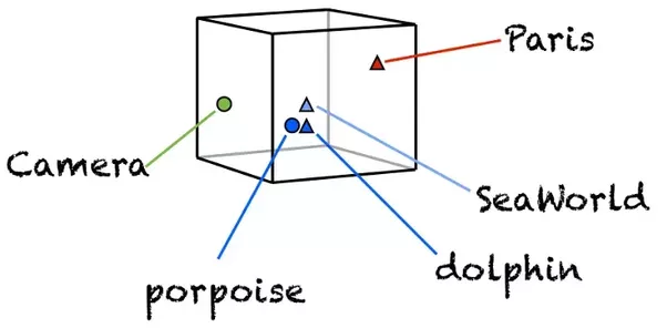
In order to be able to represent semantic proximity, it was proposed to use embedding, that is, to associate a word with a vector representing its meaning in the “space of meanings”.

What is the easiest way to get a vector from a word? It seems that it will be natural to take the vector of the length of our dictionary and put only one unit in the position corresponding to the number of the word in the dictionary. This approach is called one-hot encoding (OHE). OHE still does not have semantic proximity properties:

So we need to find another way to convert words into vectors, but OHE will still come in handy.

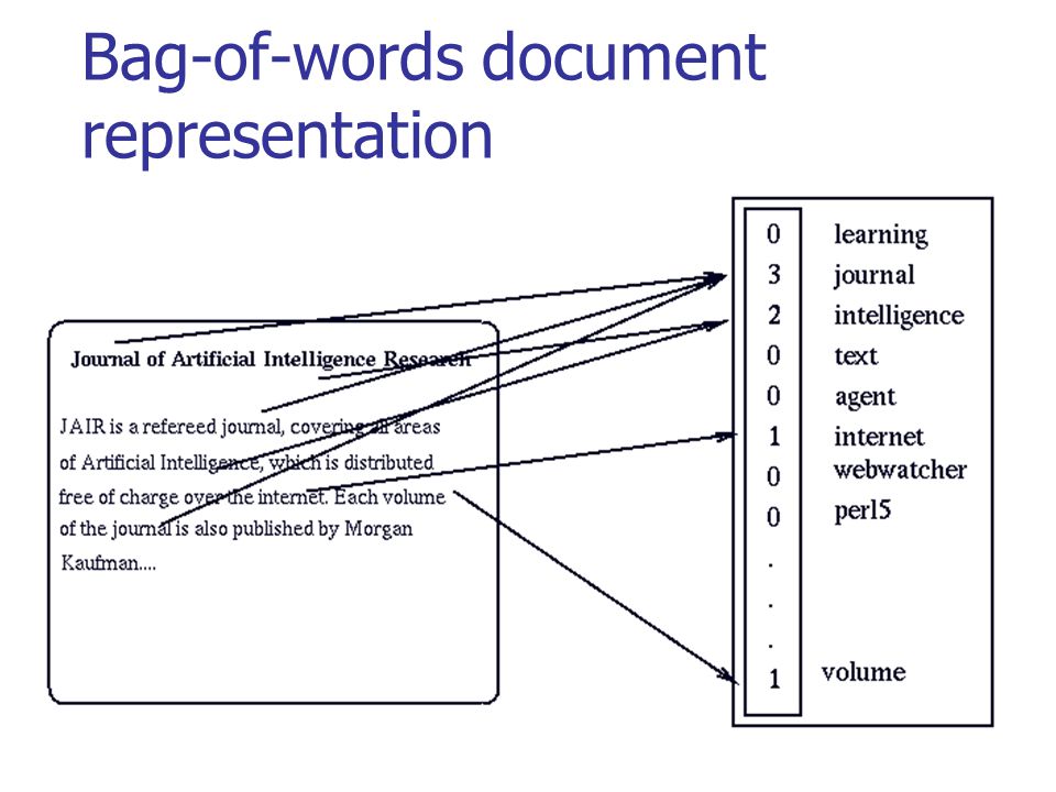
Let's step back a bit - the meaning of one word may not be so important to us, because Speech (both oral and written) consists of sets of words that we call texts. So if we want to somehow present the texts, then we take the OHE vector of each word in the text and put it together. Those. at the output we get just a count of the number of different words in the text in one vector. This approach is called “bag of words” (BoW), because we lose all the information about the relative position of words within the text.

But despite the loss of this information so the texts can already be compared. For example, using a cosine measure .

We can go further and present our corpus (set of texts) as a word-document matrix (term-document). It is worth noting that in the field of information retrieval (information retrieval), this matrix is ​​called the "reverse index" (inverted index), in the sense that a regular / direct index looks like a "document word" and is very inconvenient for a quick search. But this again goes beyond the scope of this article.

This matrix leads us to thematic models, where the word-document matrix is ​​attempted to be represented as a word-theme and subject-document product of two matrices. In the simplest case, we take the matrix and, using the SVD decomposition, we get the representation of words through themes and documents through themes:

Here $$$t_i$ - the words, $$$d_i$ - documents. But this will be the subject of another article, and now we will return to our main topic - the vector representation of words.

Suppose we have such a case:

s = ['Mars has an athmosphere', "Saturn 's moon Titan has its own athmosphere", 'Mars has two moons', 'Saturn has many moons', 'Io has cryo-vulcanoes'] 

Using the SVD transform, select only the first two components, and draw:

What is interesting in this picture? The fact that Titan and Io are far apart, although both of them are Saturn’s moons, there’s nothing in our corps. The words "atmosphere" and "Saturn" are very close to each other, although they are not synonymous. At the same time, the “two” and “many” stand side by side, which is logical. But the general meaning of this example is that the results that you get are very dependent on the case with which you work. All the code for getting the picture above can be viewed here .

The narration logic introduces the following modification of the term-document matrix, the TF-IDF formula. This abbreviation means "term frequency - inverse document frequency".

Let's try to figure out what it is. So TF is the frequency of the word. $$$w$ in the text $$$d$ , there is nothing complicated. But IDF is a much more interesting thing: it is the logarithm of the inverse of the frequency of the word $$$w$ in the case $$$C$ . The prevalence is the ratio of the number of texts in which the search word is found to the total number of texts in the corpus. With the help of TF-IDF, texts can also be compared , and this can be done with less apprehension than when using normal frequencies.

New era

The approaches described above were (and remain) good for times (or areas), where the number of texts is small and the dictionary is limited, although, as we have seen, there also have their own difficulties. But with the advent of the Internet into our life, everything became both more complicated and simpler: a great variety of texts appeared in the access, and these texts with a changing and expanding vocabulary. It was necessary to do something with this, and previously known models could not cope with such a volume of texts. The number of words in English is very roughly a million - the matrix of joint occurrences of only pairs of words will be 10 ^ 6 x 10 ^ 6. Even now, such a matrix doesn’t really crawl into the memory of computers, and, say, 10 years ago, one could not dream of such a thing. Of course, many methods were invented to simplify or parallelize the processing of such matrices, but all of these were palliative methods.

And then, as is often the case, a way out was proposed on the principle “the one who bothers us will help us!” Namely, in 2013 then little-known Czech graduate student Tomash Mikolov proposed his own approach to word embedding, which he called word2vec . His approach is based on another important hypothesis, which in science is called the locality hypothesis - “words that occur in the same environments have similar meanings”. Intimacy in this case is understood very broadly, as the fact that only matching words can stand next to each other. For example, the phrase "clockwork alarm clock" is familiar to us. And we cannot say “a clockwork orange” * - these words are not combined.

Based on this hypothesis, Tomash Mikolov proposed a new approach that did not suffer from large amounts of information, but on the contrary won [1].

The model proposed by Mikolov is very simple (and therefore so good) - we will predict the probability of a word according to its environment (context). That is, we will learn such word vectors so that the probability assigned by the model to a word is close to the probability of meeting this word in this environment in a real text.

Here $$$w_o$ - vector of the target word, $$$w_c$ Is a certain vector of context calculated (for example, by averaging) from the vectors surrounding the desired word of other words. BUT $$$s (w_1, w_2)$ Is a function that maps one number to two vectors. For example, this may be the cosine distance mentioned above.

The above formula is called softmax, that is, “soft maximum”, soft - in the sense of differentiable. This is necessary so that our model can learn using backpropagation, that is, the process of back propagation of an error.

The training process is organized as follows: we take sequentially (2k + 1) words, the word in the center is the word that should be predicted. And the surrounding words are the context of length k on each side. Each word in our model is associated with a unique vector, which we change in the process of learning our model.

In general, this approach is called CBOW - continuous bag of words, continuous, because we feed our models successively sets of words from text, and BoW because the order of words in the context is not important.

Mikolov also immediately proposed another approach - directly opposite to CBOW, which he called skip-gram, that is, “a phrase with a pass”. We are trying to guess its context from a word given to us (more precisely, a context vector). The rest of the model remains unchanged.

What is worth noting: although there is clearly no semantics in the model, but only the statistical properties of the corpus of the texts, it turns out that the trained word2vec model can capture some semantic properties of words. A classic example from the work of the author:

The word "man" refers to the word "woman" in the same way as the word "uncle" to the word "aunt", which is completely natural and understandable for us, but in other models the same ratio of vectors can be achieved only with the help of special tricks. Here - it comes naturally from the body of texts. By the way, in addition to semantic links, syntactic ones are also captured, on the right, the ratio of singular and plural numbers is shown.

More complicated things

In fact, since then, improvements have been proposed to the already classic Word2Vec model. The two most common will be described below. But this section may be omitted without prejudice to the understanding of the article as a whole, if it seems too complicated.

Negative sampling

In the standard CBoW model discussed above, we predict word probabilities and optimize them. The function for optimization (minimization in our case) is Kullback-Leibler divergence:

Here $$$p (x)$ - the probability distribution of words, which we take from the body, $$$q (x)$ - the distribution that our model generates. Divergence is literally a “divergence,” as far as one distribution is different. Since our distributions in words, i.e. are discrete, we can replace the integral with the sum in this formula:

It turned out that it is quite difficult to optimize this formula. First of all, due to the fact that $$$q (x)$ calculated using softmax throughout the dictionary. (As we remember, in English now it is of the order of a million words.) It is worth noting that many words do not occur together, as we noted above, so most of the softmax calculations are redundant. An elegant workaround called Negative Sampling was proposed. The essence of this approach is that we maximize the probability of encountering the right word in a typical context (one that is often found in our corpus) and at the same time minimize the probability of a meeting in an atypical context (one that is rarely or not at all). The formula above is written like this:

Here $$$s (x, w)$ - Exactly the same as in the original formula, but the rest is somewhat different. First of all, you should pay attention to the fact that the formula now consists of two parts: positive ( $$$s (x, w)$ ) and negative ( $$$-s (x, w)$ ). The positive part is responsible for typical contexts, and $$$D$ here is the distribution of co-occurrence of the word $$$w$ and the rest of the words of the body. The negative part - this is perhaps the most interesting - this is a set of words that are rarely found with our target word. This set is generated from the distribution $$$D '$ which in practice is taken as uniform over all the words of the hull dictionary. It was shown that such a function leads, with its optimization, to a result similar to the standard softmax [2].

Hierarchical softmax

Also, people came in from the other side - you can not change the original formula, but try to count the softmax itself more efficiently. For example, using a binary tree [3]. For all the words in the dictionary is built Huffman tree. In the resulting tree $$$V$ Words are located on the leaves of the tree.

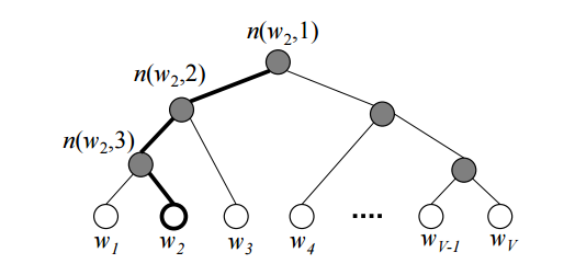
The figure shows an example of such a binary tree. Bold highlighted path from the root to the word $$$w_2$ . The length of the path denote $$$L (w)$ , but $$$j$ top on the way to the word $$$w$ denote by $$$n (w, j)$ . It can be proved that inner vertices (not leaves) $$$V - 1$ .

Using hierarchical softmax vector $$$v_ {n (w, j)}$ predicted for $$$V-1$ internal vertices. And the probability that the word $$$w$ will be the output word (depending on what we predict: a word from the context or a given word according to the context) is calculated by the formula:

$$$p (w = w_o) = \ prod \ limits_ {j = 1} ^ {L (w) -1} \ sigma ([n (w, j + 1) = lch (n (w, j))] v_ {n (w, j)} ^ T u)$

Where $$$\ sigma (x)$ - softmax function; $$$[true] = 1, [false] = - 1$ ; $$$lch (n)$ - left son of the top $$$n$ ; $$$u = v_ {w_I}$ , if skip-gram is used, $$$u = \ frac {1} {h} \ sum \ limits_ {k = 1} ^ {h} v_ {w_ {I, k}}$ that is, the averaged context vector, if CBOW is used.

The formula can be intuitively understood by imagining that at every step we can go left or right with probabilities:

$$$p (n, left) = \ sigma (v_n ^ T u)$
$$$p (n, right) = 1-p (n, left) = 1- \ sigma (v_n ^ T u) = \ sigma (-v_n ^ T u)$

Then, at each step, the probabilities are multiplied together ( $$$L (w) -1$ steps) and it turns out the desired formula.

When using simple softmax to calculate the probability of a word, it was necessary to calculate the normalizing sum for all words from the dictionary, it was required $$$O (v)$ operations. Now, the probability of the word can be calculated using successive calculations that require $$$O (log (V))$ .

Other models

In addition to word2vec, other word embedding models were proposed, of course. It is worth noting the model proposed by the laboratory of computational linguistics at Stanford University, called Global Vectors (GloVe), combining the features of SVD decomposition and word2vec [4].

Also it is necessary to mention that since Initially, all the described models were proposed for the English language, then the inflection problem typical for synthetic languages ​​(this is a linguistic term ), such as Russian, is not so acute. Everywhere above, it was implicitly assumed that we either consider different forms of the same word as different words - and then we hope that our corps will be enough for the model to learn their syntactic proximity, or we use the mechanisms of stemming or lemmatization. Stemming is the cutting off of the end of a word, leaving only the stem (for example, a “red apple” will turn into “red apples”). And lemmatization - replacing a word with its initial form (for example, “we run” will turn into “I run”). But we can not lose this information, and use it - by coding OHE into a new vector, and converting it with a vector for a basis or a lemma.
It is also worth saying that what we started with - the literal representation of the word - also did not sink into oblivion: models for using the literal representation of the word for the word embedding were proposed [5].

Practical use

We talked about the theory, it's time to see what all of the above is applicable in practice. After all, any of the most beautiful theory without practical application is nothing more than a play of the mind. Consider the use of Word2Vec in two tasks:
1) The task of classification, it is necessary to identify the user by the sequence of visited sites
2) The task of regression, it is necessary in the text of the article to determine its rating on Habrahabr.

Classification

 #      from __future__ import division, print_function #    Anaconda import warnings warnings.filterwarnings('ignore') #%matplotlib inline import numpy as np import pandas as pd from sklearn.metrics import roc_auc_score 

You can download data for the first task from the page of the competition "Catch Me If You Can"

 #      train_df = pd.read_csv('data/train_sessions.csv')#,index_col='session_id') test_df = pd.read_csv('data/test_sessions.csv')#, index_col='session_id') #   time1, ..., time10    times = ['time%s' % i for i in range(1, 11)] train_df[times] = train_df[times].apply(pd.to_datetime) test_df[times] = test_df[times].apply(pd.to_datetime) #     train_df = train_df.sort_values(by='time1') #      train_df.head()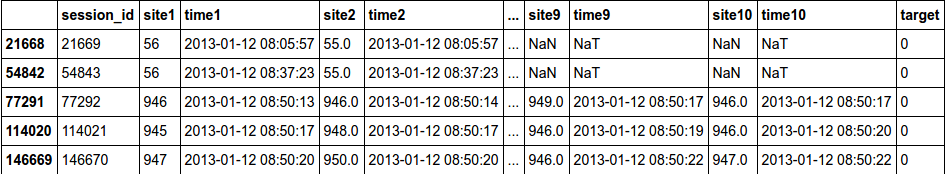 

 sites = ['site%s' % i for i in range(1, 11)] # nan  0 train_df[sites] = train_df[sites].fillna(0).astype('int').astype('str') test_df[sites] = test_df[sites].fillna(0).astype('int').astype('str') #     word2vec train_df['list'] = train_df['site1'] test_df['list'] = test_df['site1'] for s in sites[1:]: train_df['list'] = train_df['list']+","+train_df[s] test_df['list'] = test_df['list']+","+test_df[s] train_df['list_w'] = train_df['list'].apply(lambda x: x.split(',')) test_df['list_w'] = test_df['list'].apply(lambda x: x.split(',')) 

 #      ,    #      , ..        . train_df['list_w'][10] 

 ['229', '1500', '33', '1500', '391', '35', '29', '2276', '40305', '23'] 

 #  word2vec from gensim.models import word2vec 

 #            #    6=3*2 (  10 )     300,  workers     test_df['target'] = -1 data = pd.concat([train_df,test_df], axis=0) model = word2vec.Word2Vec(data['list_w'], size=300, window=3, workers=4) #        w2v = dict(zip(model.wv.index2word, model.wv.syn0)) 

Since Now we have compared a vector to each word, then we need to decide what to associate with the whole sentence of words.
One of the possible options is simply to average all the words in the sentence and get some meaning for the whole sentence (if the word is not in the text, then we take the zero vector).

 class mean_vectorizer(object): def __init__(self, word2vec): self.word2vec = word2vec self.dim = len(next(iter(w2v.values()))) def fit(self, X): return self def transform(self, X): return np.array([ np.mean([self.word2vec[w] for w in words if w in self.word2vec] or [np.zeros(self.dim)], axis=0) for words in X ]) 

 data_mean=mean_vectorizer(w2v).fit(train_df['list_w']).transform(train_df['list_w']) data_mean.shape 

 (253561, 300) 

Since we got distributed representation, then no number individually means nothing, which means best linear algorithms will show themselves. Let's try neural networks, LogisticRegression and check the non-linear method XGBoost.

 #   def split(train,y,ratio): idx = round(train.shape[0] * ratio) return train[:idx, :], train[idx:, :], y[:idx], y[idx:] y = train_df['target'] Xtr, Xval, ytr, yval = split(data_mean, y,0.8) Xtr.shape,Xval.shape,ytr.mean(),yval.mean() 

 ((202849, 300), (50712, 300), 0.009726446765820882, 0.006389020350212968) 

 #   keras from keras.models import Sequential, Model from keras.layers import Dense, Dropout, Activation, Input from keras.preprocessing.text import Tokenizer from keras import regularizers 

 #    model = Sequential() model.add(Dense(128, input_dim=(Xtr.shape[1]))) model.add(Activation('relu')) model.add(Dropout(0.5)) model.add(Dense(1)) model.add(Activation('sigmoid')) model.compile(loss='binary_crossentropy', optimizer='adam', metrics=['binary_accuracy']) 

 history = model.fit(Xtr, ytr, batch_size=128, epochs=10, validation_data=(Xval, yval), class_weight='auto', verbose=0) 

 classes = model.predict(Xval, batch_size=128) roc_auc_score(yval, classes) 

 0.91892341356995644 

Got a good result. So Word2Vec was able to identify the dependencies between the sessions.
Let's see what happens with the XGBoost algorithm.

 import xgboost as xgb 

 dtr = xgb.DMatrix(Xtr, label= ytr,missing = np.nan) dval = xgb.DMatrix(Xval, label= yval,missing = np.nan) watchlist = [(dtr, 'train'), (dval, 'eval')] history = dict() 

 params = { 'max_depth': 26, 'eta': 0.025, 'nthread': 4, 'gamma' : 1, 'alpha' : 1, 'subsample': 0.85, 'eval_metric': ['auc'], 'objective': 'binary:logistic', 'colsample_bytree': 0.9, 'min_child_weight': 100, 'scale_pos_weight':(1)/y.mean(), 'seed':7 } 

 model_new = xgb.train(params, dtr, num_boost_round=200, evals=watchlist, evals_result=history, verbose_eval=20) 

 [0] train-auc:0.954886 eval-auc:0.85383 [20] train-auc:0.989848 eval-auc:0.910808 [40] train-auc:0.992086 eval-auc:0.916371 [60] train-auc:0.993658 eval-auc:0.917753 [80] train-auc:0.994874 eval-auc:0.918254 [100] train-auc:0.995743 eval-auc:0.917947 [120] train-auc:0.996396 eval-auc:0.917735 [140] train-auc:0.996964 eval-auc:0.918503 [160] train-auc:0.997368 eval-auc:0.919341 [180] train-auc:0.997682 eval-auc:0.920183 

We see that the algorithm is strongly adapted to the training sample, so it is possible that our assumption about the need to use linear algorithms has been confirmed.
Let's see what the usual LogisticRegression will show.

 from sklearn.linear_model import LogisticRegression def get_auc_lr_valid(X, y, C=1, seed=7, ratio = 0.8): #       idx = round(X.shape[0] * ratio) #   lr = LogisticRegression(C=C, random_state=seed, n_jobs=-1).fit(X[:idx], y[:idx]) #     y_pred = lr.predict_proba(X[idx:, :])[:, 1] #   score = roc_auc_score(y[idx:], y_pred) return score 

 get_auc_lr_valid(data_mean, y, C=1, seed=7, ratio = 0.8) 

 0.90037148150108237 

Let's try to improve the results.

Now, instead of the usual average, to take into account the frequency with which the word occurs in the text, take the weighted average. We take IDF as weights. Accounting for IDF reduces the weight of widely used words and increases the weight of more rare words that can quite accurately indicate which class the text belongs to. In our case, who owns the sequence of visited sites.

 #   tfidf . from sklearn.feature_extraction.text import TfidfVectorizer from collections import defaultdict class tfidf_vectorizer(object): def __init__(self, word2vec): self.word2vec = word2vec self.word2weight = None self.dim = len(next(iter(w2v.values()))) def fit(self, X): tfidf = TfidfVectorizer(analyzer=lambda x: x) tfidf.fit(X) max_idf = max(tfidf.idf_) self.word2weight = defaultdict( lambda: max_idf, [(w, tfidf.idf_[i]) for w, i in tfidf.vocabulary_.items()]) return self def transform(self, X): return np.array([ np.mean([self.word2vec[w] * self.word2weight[w] for w in words if w in self.word2vec] or [np.zeros(self.dim)], axis=0) for words in X ]) 

 data_mean = tfidf_vectorizer(w2v).fit(train_df['list_w']).transform(train_df['list_w']) 

Check whether the quality of the LogisticRegression has changed.

 get_auc_lr_valid(data_mean, y, C=1, seed=7, ratio = 0.8) 

 0.90738924587178804 

we see a gain of 0.07, which means that the weighted average probably helps to better reflect the meaning of the whole sentence through word2vec.

Prediction of popularity

Let's try Word2Vec already in a text task - predicting the popularity of an article on Khabrhabr.

Let's try the algorithm forces directly on the text data of Habr's articles. We converted the data to a csv table. You can download them here: train , test .

 Xtrain = pd.read_csv('data/train_content.csv') Xtest = pd.read_csv('data/test_content.csv') print(Xtrain.shape,Xtest.shape) Xtrain.head() 

. .

, Word2Vec.
, .

1) ;

2) ;

3) , .. ;

4) , — () .

.

 #    from sklearn.metrics import mean_squared_error import re from nltk.corpus import stopwords import pymorphy2 morph = pymorphy2.MorphAnalyzer() stops = set(stopwords.words("english")) | set(stopwords.words("russian")) def review_to_wordlist(review): #1) review_text = re.sub("[^--a-zA-Z]"," ", review) #2) words = review_text.lower().split() #3) words = [w for w in words if not w in stops] #4) words = [morph.parse(w)[0].normal_form for w in words ] return(words) 

, .

 #   Xtrain['date'] = Xtrain['date'].apply(pd.to_datetime) Xtrain['year'] = Xtrain['date'].apply(lambda x: x.year) Xtrain['month'] = Xtrain['date'].apply(lambda x: x.month) 

2015 , 4 2016, .. 4 2017 . , ,

 Xtr = Xtrain[Xtrain['year']==2015] Xval = Xtrain[(Xtrain['year']==2016)& (Xtrain['month']<=4)] ytr = Xtr['favs_lognorm'] yval = Xval['favs_lognorm'] Xtr.shape,Xval.shape,ytr.mean(),yval.mean() 

 ((23425, 15), (7556, 15), 3.4046228249071526, 3.304679829935242) 

 data = pd.concat([Xtr,Xval],axis = 0,ignore_index = True) 

 #   nan,      data['content_clear'] = data['content'].apply(str) 

 %%time data['content_clear'] = data['content_clear'].apply(review_to_wordlist) 

 model = word2vec.Word2Vec(data['content_clear'], size=300, window=10, workers=4) w2v = dict(zip(model.wv.index2word, model.wv.syn0)) 

:

 model.wv.most_similar(positive=['open', 'data','science','best']) 

, :

 data_mean = mean_vectorizer(w2v).fit(data['content_clear']).transform(data['content_clear']) data_mean.shape 

 def split(train,y,ratio): idx = ratio return train[:idx, :], train[idx:, :], y[:idx], y[idx:] y = data['favs_lognorm'] Xtr, Xval, ytr, yval = split(data_mean, y,23425) Xtr.shape,Xval.shape,ytr.mean(),yval.mean() 

 ((23425, 300), (7556, 300), 3.4046228249071526, 3.304679829935242) 

 from sklearn.linear_model import Ridge from sklearn.metrics import mean_squared_error model = Ridge(alpha = 1,random_state=7) model.fit(Xtr, ytr) train_preds = model.predict(Xtr) valid_preds = model.predict(Xval) ymed = np.ones(len(valid_preds))*ytr.median() print('  ',mean_squared_error(ytr, train_preds)) print('  ',mean_squared_error(yval, valid_preds)) print('    ',mean_squared_error(yval, ymed)) 

    0.734248488422    0.665592676973      1.44601638512 

 data_mean_tfidf = tfidf_vectorizer(w2v).fit(data['content_clear']).transform(data['content_clear']) 

 y = data['favs_lognorm'] Xtr, Xval, ytr, yval = split(data_mean_tfidf, y,23425) Xtr.shape,Xval.shape,ytr.mean(),yval.mean() 

 ((23425, 300), (7556, 300), 3.4046228249071526, 3.304679829935242) 

 model = Ridge(alpha = 1,random_state=7) model.fit(Xtr, ytr) train_preds = model.predict(Xtr) valid_preds = model.predict(Xval) ymed = np.ones(len(valid_preds))*ytr.median() print('  ',mean_squared_error(ytr, train_preds)) print('  ',mean_squared_error(yval, valid_preds)) print('    ',mean_squared_error(yval, ymed)) 

    0.743623730976    0.675584372744      1.44601638512 

.

 #   keras from keras.models import Sequential, Model from keras.layers import Dense, Dropout, Activation, Input from keras.preprocessing.text import Tokenizer from keras import regularizers from keras.wrappers.scikit_learn import KerasRegressor 

 #   . def baseline_model(): model = Sequential() model.add(Dense(128, input_dim=Xtr.shape[1], kernel_initializer='normal', activation='relu')) model.add(Dropout(0.2)) model.add(Dense(64, activation='relu')) model.add(Dropout(0.5)) model.add(Dense(1, kernel_initializer='normal')) model.compile(loss='mean_squared_error', optimizer='adam') return model estimator = KerasRegressor(build_fn=baseline_model,epochs=20, nb_epoch=20, batch_size=64,validation_data=(Xval, yval), verbose=2) 

 estimator.fit(Xtr, ytr) 

.

Conclusion

Word2Vec , - — — GloVe. , , , , word2vec.

. — .

demonzheg .

Literature

1. Tomas Mikolov, Kai Chen, Greg Corrado, and Jeffrey Dean. Efficient estimation
   of word representations in vector space. CoRR, abs/1301.3781,
2. Tomas Mikolov, Ilya Sutskever, Kai Chen, Gregory S. Corrado, and Jeffrey Dean. Distributed representations of words and phrases and their compositionality. In Advances in Neural Information Processing Systems 26: 27th Annual Conference on Neural Information Processing Systems 2013. Proceedings of a meeting held December 5-8, 2013, Lake Tahoe, Nevada, United States, pages 3111–3119, 2013.
3. Morin, F., & Bengio, Y. Hierarchical Probabilistic Neural Network Language Model . Aistats, 5, 2005.
4. Jeffrey Pennington, Richard Socher, and Christopher D. Manning. GloVe: Global Vectors for Word Representation. 2014.
5. Piotr Bojanowski, Edouard Grave, Armand Joulin, and Tomas Mikolov. Enriching word vectors
   with subword information. arXiv preprint arXiv:1607.04606, 2016.

* , .