Genetic Advisor for Options Trading

When trading options, one of the main tasks is to determine the fair price of the option. Based on it, one can understand which options are undervalued by the market, and which are overvalued at the moment. Based on this, decisions are made on the purchase or sale of a specific option. This article discusses the experience of creating an adviser based on the Genetic Algorithm (GA), which allows to automate the process of choosing options for sale and purchase, respectively. The Advisor, unlike trading robots (or Mechanical Trading Systems MTS), does not make only gives recommendations to the trader, who already independently decides to make a deal or not.

First, a few words about the genetic algorithm:
')
It makes no sense to describe the genetic algorithm in detail, since this topic is well presented both on this resource and in general on the Internet. I will dwell only on the main points that are necessary to understand the concept of a genetic advisor as a whole.

So, the genetic algorithm can be viewed as a directed, random search for the optimal solution of any problem. For example, consider the target function of the form:

$$$$ display $$ S = F (X_1, X_2, ... X_n) (1) $$ display $$

Where: S is the value of the function F from several arguments X1..Xn.

Suppose that all arguments X lie in a certain range of integer values ​​from -100 to 100. To find the maximum (optimal) value of S, it is necessary to choose such a combination of arguments X at which the function F will be maximal. With a small number of arguments, the problem can be solved analytically, but with an increase in the number of arguments, the complexity of such a solution increases significantly. Theoretically, the problem can be solved by the method of enumerating possible solutions, provided that all arguments X are integer. However, with the range of arguments from -100 to 100 and the number of arguments 10, the number of possible solutions is approximately equal to

$$$$ display $$ 1.076 * 10 ^ {23} $$ display $$

If we assume that it takes 1 nanosecond to calculate one option, then it will take several million years for a computer to iterate through all the options! Those. brute force solution in this form is not viable. This is where the genetic algorithm comes to the rescue, the essence of which lies in the fact that all the arguments of the function are encoded in binary form. For coding one argument with a range of -100: 100 (or 201 possible values) we need 8 bits (one gene),$$ $ inline $ 2 ^ 8 = 256 $ inline $ (the nearest binary value is greater than 201), so we need to use 80 bits to encode all 10 arguments. This binary sequence is called a genotype (chromosome) (the genetic algorithm uses terms from biology). Initially, a population of random genotypes is created. Those. in our case, several binary sequences are created (say, 20), each of which is 80 bits long and which are filled with 0 and 1 randomly.

Next, for each individual (binary sequence), we calculate the value of the function and select those individuals that show the maximum values ​​(for example, the first 10 maximum values ​​out of 20) of the objective function (the analogue of natural selection, those who are most adapted survive). For selected individuals, we carry out the procedure of crossing, mutation, and create a new generation of individuals, which are already more adapted than the initial population, from which we again select the most adapted individuals. Conducting such a cycle several times we consistently “grow” a genotype that brings us closer to the maximum value of the objective function. It is worth noting that there are a lot of variants of selection, crossing and mutation of genotypes, in addition there is the problem of local maxima, population degeneration, but these issues are beyond the scope of this article and are recommended for independent study.

Options

Options are derivative financial instruments with non-linear value. At the core of options is Basic Asset (BA). Options are of 2 types of CALL options, the cost of which increases with the GROWTH of the BA price and the PUT options, the cost of which increases when the price of BA is REDUCED. To calculate the theoretical option price, use the famous Black-Scholes formula. In the Russian market of BA for options is the corresponding futures. So for options on the US dollar, BA is futures (Si) on the US dollar. Options, as well as futures, have a lifespan. The date when the option ends its existence is called the expiration date. At this point, the final payment is made on the options that the trader has in the basket.

Despite the complexity of these instruments, they have properties that other financial instruments do not have. One of these features is that they essentially allow you to simultaneously trade one and the same tool (underlying asset) but at different expected prices (strikes), this makes it possible to build complex combinations of options of different types (CALL / PUT) and different prices (strikes).

Conventionally, options trading can be divided into 2 types: static and dynamic.

In static trading, the trader makes some assumptions about the price of BA in the future, and depending on this builds a position. For example, if a trader believes that the price will remain in a certain range, then he can sell CALL and PUT options and earn on the received premium from the sale. However, if the price of a BA approaches the edge of such a position, then it must be “regulated” so as not to get a loss.

In dynamic trading, the bet is not on a specific BA price movement, but on price fluctuation, i.e. volatility. With high volatility, option prices can change significantly, which makes it possible to make money.

The considered concept of options trading with the help of GA refers to static trading, on which we dwell in more detail.

"Cheap" and "Dear" options

So, imagine a trader who makes the assumption that the US dollar will rise in price in the near future and he wants to make money on it using the option position. The trader buys 10 CALL options with a strike of 56000 at a price of 1,800 rubles per option. In this case, the position of the trader will have the form shown in Fig.1.


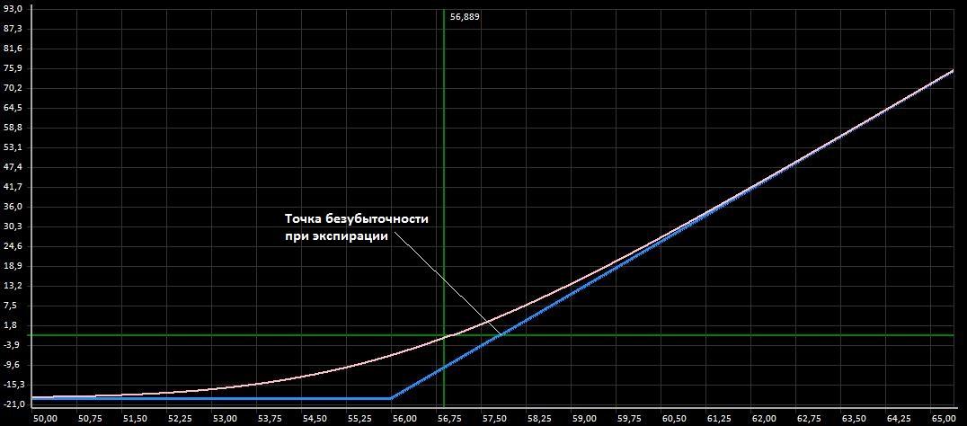
Fig.1. Purchased CALL Options

From which it is clear that the position will be profitable if, at the time of expiration, the BA price will be more than 57,800, otherwise the position will be unprofitable, and the maximum loss will be 18,000 rubles. To reduce the maximum loss, the trader decides to sell 10 more CALL options with a strike of 58,000 at a price of 905 rubles. In this case, the position will be presented in Fig.2. This position is called the bullish CALL Spread.


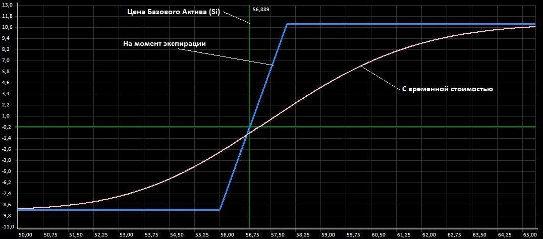
Fig.2. Bullish CALL Spread

The maximum loss is reduced to 8,950 rubles, but at the same time the maximum profit becomes limited, the break-even point shifts to the left.

Now imagine that options with a strike of 56,000 are overvalued by the market and were bought at a price of 2,000 rubles, and options with a strike of 58,000, on the contrary, are underestimated and sold for 700 rubles, then the position will look like:


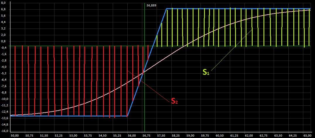
Fig.3. Bought more, sold cheaper

Consider the opposite situation, when the trader was able to buy options cheaper (1500 rubles) and sell more expensive (1200 rubles) then the position would look like:


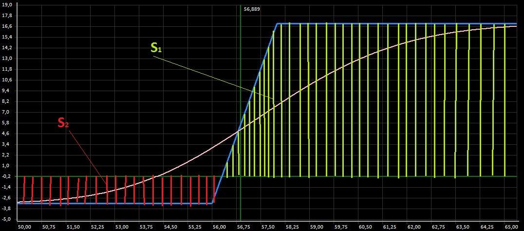
Fig.4. Bought cheaper, sold more expensive.

Analyzing the graphs in Figures 2.3 and 4, it becomes obvious that the “positive” area of ​​the S1 graph increases, and the “negative” S2 decreases in proportion to the cheaper options we buy and sell more expensive. In other words, trying to buy undervalued (cheap) options and sell overvalued (expensive) ones, we increase the “positive” area of ​​the position –S1 and decrease the “negative” area - S2. Thus, the quality of the option position can be formally assessed by the size of the area S1. The ideal case when S1 is maximal and S2 is completely absent.

In addition, it is possible to hypothesize that, with a limited amount of Guarantee Security (GO) position and a given range of strikes, at any given time there is theoretically such a combination of purchased and sold options where the “positive” area of ​​the position will be maximum .

In general, a “positive” area can be represented as a function of the sum of the areas of purchased and sold options of different strikes:

$$$$ display $$ S_1 = F (X_1, X_2 ... X_n) (2) $$ display $$

Where: X1..Xn - the number of sold / purchased options on each strike

It is easy to see that the area function S1 (2) corresponds to the objective function GA (1) considered above. Those. applied to the option position, the size of the “positive” area will be the objective function. To find the maximum possible "positive" area of ​​a position with GO, for example, not more than 100,000 rubles, you can sort through all possible combinations of options, however, as was shown earlier, it takes a disastrously long time, therefore using GA to search for the optimal position positive "area) is fully justified.

It is necessary to add that this approach can be used not only to form the initial position, but also to regulate the existing one. Since prices in the market change all the time, this situation may arise when buying or selling options will lead to an increase in the “positive” area of ​​the current position. In this case, the objective function will be:

$$$$ display $$ S_1 = F_0 (Z_1, Z_2, ... Z_k) + F (X_1, X_2, ... X_n) (3) $$ display $$

Where: F0 is a function of the sum of the areas of the existing position, Z1..Zk is the number of sold / purchased options on each strike.

Implementation

Thus, the main function of the adviser is to search for such a combination of purchased / sold options where the “positive” area of ​​the position will be maximum for a given length of one gene, i.e. while limiting the maximum number of options for one strike.

Advisor itself is written in C # language which performs all calculations. The Expert Advisor obtains the initial data for the calculations from the QUIK terminal using a module written in Lua and a connector written in C ++. See fig.5.


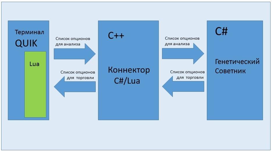
Fig.5. The structural diagram of the adviser.

The Lua module analyzes the prices of options and transfers them to the advisor, and it makes no sense to use all possible strikes since there are almost no “lives” on many strikes (for example, on very distant strikes). Therefore, only those options that can be bought or sold with a high probability are used for analysis. After calculations, the adviser sends the list of options for buying / selling back to QUIK, where the same module on Lua places bids and controls their execution.

The functionality of the advisor allows you to build a graph of the current position, perform a genetic search for the optimal position, adjust the result manually, if necessary, transfer data for trading back to QUIK. The advisor view is shown in Fig.6a. and 6c.


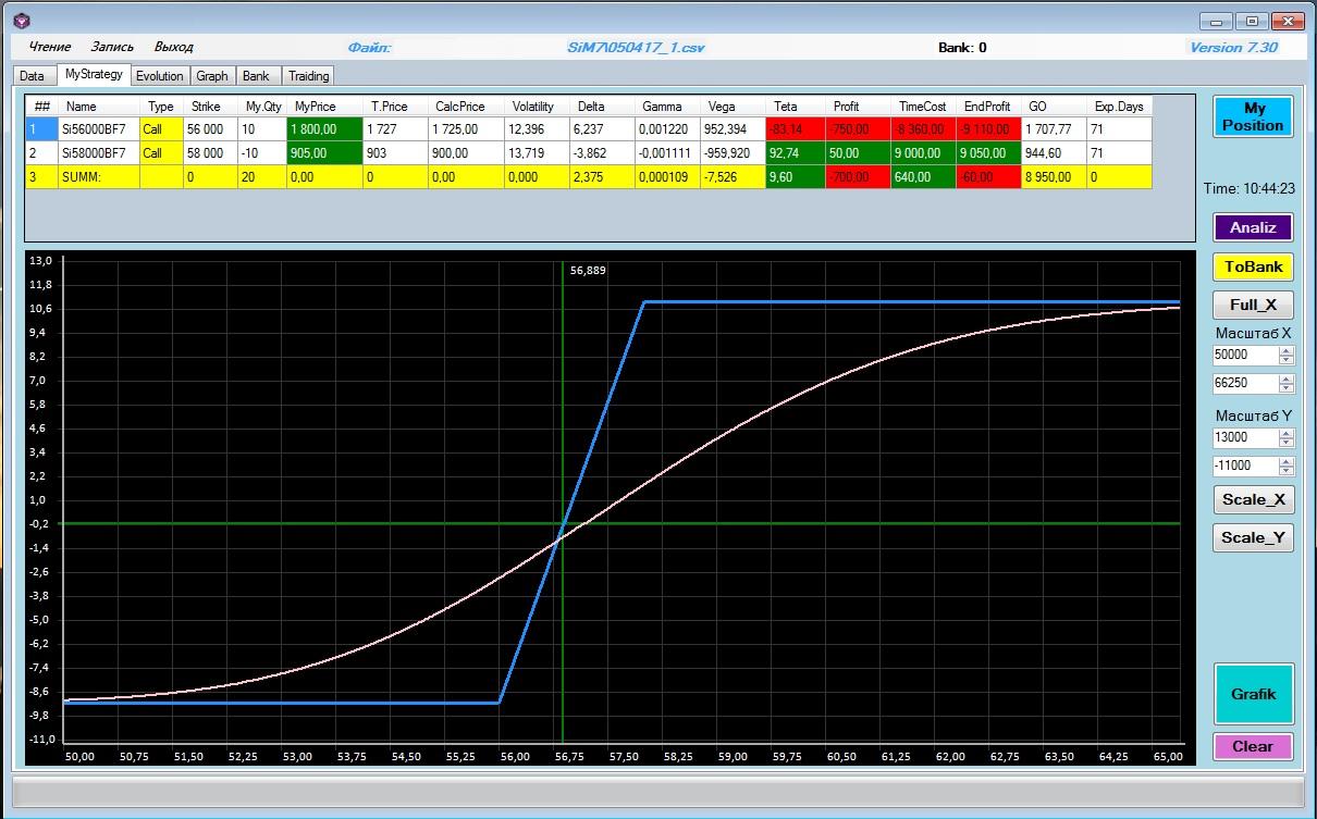
Fig.6a. Genetic Advisor Interface


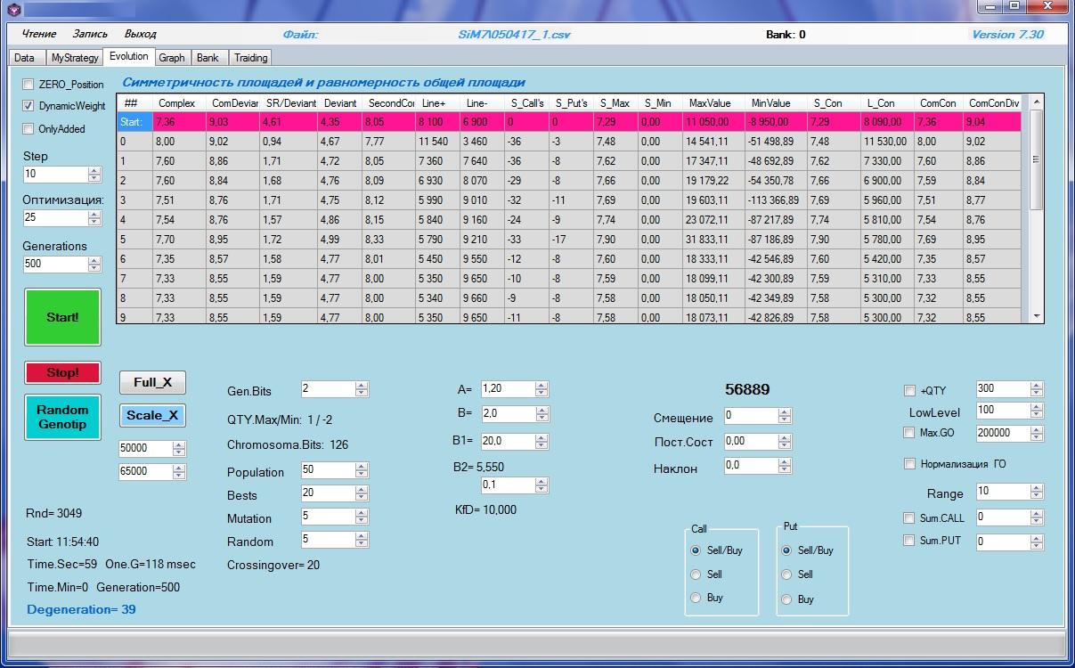
Fig.6b. Genetic Algorithm Settings.

More about the objective function

We have chosen the “positive” position area as the target function, but this approach does not fully reflect the “quality” of the option position. Where quality is the ratio of return / risk. For example, with a sufficiently large “positive” area, the “negative” area may be even larger. Or, for example, the “positive” area can be pulled up. Those. the objective function must be made more “smart” so that it reflects the quality of the position more effectively. One simple option is to use the ratio of "positive" and "negative" areas - S1 / S2. In this variant, the objective function will increase with an increase in the positive area (yield) and with a decrease in the “negative” (risk).

The first "pitfalls"

To assess the work of the adviser, let us take the CALL-spread created position (Fig. 2) and try to improve it with the help of the adviser. After 1000 generations we get a new position - Fig.7.


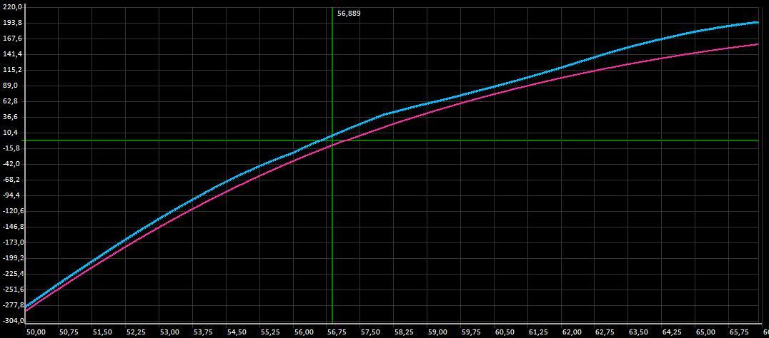
Fig.7. The first result of the work of the GA.

The result, to put it mildly, is not impressive, although the GA formally fulfilled its function with the size of a “positive” area larger than a “negative” one. The position became vaguely reminiscent of purchased synthetic futures. The resulting graph is explained quite simply. The fact is that for GA there is no difference in which area of ​​the chart the “positive” area is located - on distant strikes or on neighbors. But for real trading it is important that the “positive” area be concentrated near the current BA price. Since the probability of a price change by a small amount is higher than a strong price movement (unless, of course, a bet on a strong movement was initially made). In this regard, it is necessary to change the calculation of the objective function so that the area near the BA price would have more weight than the area on the long strike. To do this, we will enter into the calculation of the target function a dynamic weighting factor, Ks, which takes into account the location of the area relative to the current BA price. The area, in fact, is an integral of the function, which is calculated in this case by the method of rectangles. In the calculation, at each point the value of the area of ​​one rectangle will be multiplied by this coefficient. We take the sigmoid (logistic) function as the basis of the coefficient but make it symmetrical with respect to the current BA price:

$$$$ display $$ Ks (Strike) = 1 / (1 + e ^ {Ax-B}) (4) $$ display $$

Where: A-coefficient of the steepness of the sigmoid function, B-coefficient of "width" - are chosen empirically.

x (Strike) - the argument of the sigmoid function is calculated as:

$$$$ display $$ x = ABS ((Strike Price) / (Strike Step)) (5) $$ display $$

Obviously, the value of distant strikes will fall as the expiration date approaches. With a current BA price of 56000 points and 90 days before expiration, it is likely that the price over 90 days may increase to 65000 points or fall to 45000. But if, for example, 2 days remain before expiration, then the probability of reaching the price level is 65000 or 45000 from the current price of 56,000 is significantly reduced. Therefore, the dynamic coefficient should take into account the time before expiration, as well as the level of current volatility.

This can be done by adding to the formula a well-known coefficient taking into account both of these parameters:

$$$$ display $$ Volatility / √ {Number of days. before. expiration} (6) $$ display $$

As a result, we obtain a family of symmetric sigmoid functions depending on the time before expiration and volatility. Fig.8.


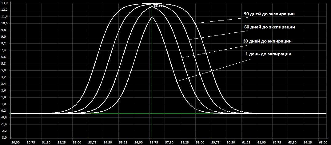
Fig.8. The family of symmetric sigmoid functions with different expiration dates (for one value of volatility)

Now, the objective function is configured so that it would give preference to the area which is near the BA price, taking into account the time to expiration and the current volatility. After such a change, the effectiveness of the position improved significantly. In Fig.9. shows the result of the advisor


Fig.9. The initial position and the position formed by the GA when using the dynamic coefficient Ks.

As a result of the work of the GA, to the originally 20 contracts, 52 new contracts were added (30 different options), the basket now consists of 72 contracts, GO about 37,000 rubles. The position has become more interesting - on the left side there is no negative area at all, i.e. when the BA price goes down, the position remains in positive territory. The right-hand side has a profit limit, and when the BA price is above 61500, the position will become negative, however, if the BA price increases, you can re-find a better position.

In addition, if we substitute not the current BA price instead of the expected one in formula (5) instead of the BA price, then the focus of our objective function will be shifted exactly to the expected area. Assume that the price of BA will increase, based on expectations, we will substitute the value 58889 into formula (5) (2,000 points more than the current price).

Then the graph of the sigmoid function and the result obtained will look like in Fig.10.


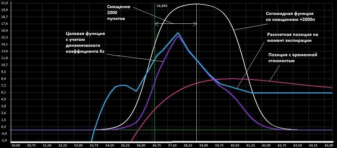
Fig.10. GA operation with 2000 point biased sigmoid function

The figure shows that the new position has changed, now we have no negative area on the right. Thus, using the coefficients A, B and the BA price shift, it is possible to build a new position with an emphasis in the area of ​​interest.

The families of positions of successively formed GAs with different displacements of the sigmoid function on the same source data are shown in Fig.11.


Figure 11. A family of positions with different offsets for the BA price.

Once again about the objective function and limitations

The form of the positions in Fig.11. differs from the previous ones, because another objective function is used. As practice has shown, the creation of an objective function is the most difficult task - it is it that determines the result. The same objective function can produce different results in different market conditions. Therefore, the ability to select various objective functions taking into account several factors has been added to the advisor: the area ratio S1 / S2, the ratio of the lengths of areas where the area is positive, the area continuity, the uniformity of area distribution, etc. In addition, the adviser allows you to impose some restrictions on the position, for example, the maximum size of the GO, the number of sold (purchased) options, etc.

findings

Practical tests of the adviser give reason to believe that the presented concept of creating an option position is fully entitled to life. Real tests have shown the ability of the adviser to create effective strategies.

The advantages of such a system include the automated formation and regulation of the position. GA allows you to get very "beautiful" positions of options that are extremely difficult to obtain with "manual" trading (due to the complex combination of a large number of different options). GA gives a fairly high convergence. If you hold a position formation several times on the same data, the results will be close to each other.

However, the advisor takes time to form a position. GA does not work so fast, especially with a large number of options and a long chromosome. In addition, sometimes it is necessary to sort out different versions of target functions in order to build an acceptable position in a specific market situation. During this time, the data on the basis of which the position is built may lose relevance. Therefore, the performance of the computer here comes out on top.

The biggest problem is the situation when the expiration is already close, and the price of BA is at the edge of the position. In this case, the regulation of the position becomes difficult because of the sharp reduction in the number of options that can be used. Although the GA copes with this task, it turns out to be risky positions with the high cost of HE. In fairness, it should be noted that such a problem exists in the hands trade.

Thanks to everyone who read to the end!