Python PID Controller Model
Looking for a simple PID controller model with an object
A large number of publications in the network are devoted to modeling the operation of the PID controller. Leading the design of PID controller models using Matlab Simulink [1,2] (134 million links in yandex). The process of creating a model is some kind of uniform. All new and new blocks are transferred to the model. One movement of the manual manipulator and here you are a PID controller, another one and that is the transfer function of the object. You connect the blocks, adjust the parameters, prepare the calculator. Yes, there are many possibilities, but somehow everything is too artificial. And it becomes completely incomprehensible to what here the differential equations, the methods for their solution and the operational calculus with which they have long wondered. I am looking for the implementation of the PID in Mathcad, there are links in the same yandex, smaller, only 81 million, and more mathematics and formulas. I look at the PID example that comes with the Mathcad 14 package.

As an object oscillatory link. Many clever explanations, but as a result two operators laplace and invlaplace. The total transfer function is in the numerator of the second degree of the operator, and in the denominator of the fourth. In order for the laplace and invlaplace operators to work when all three components of the PID are connected, the roots of the denominator of the transfer function are also found, these roots are complexly conjugate.

')
Now looking for a PID implementation in Python. Quietly rejoiced at 97 million results, but not for long. About Python 2.7 only in relation to the Arduino firmware on the example of ESP32. But this also overwhelms the heart with pride in Python.
Disappointed in the search, I decided to write the model myself, to the best of my more than modest possibilities.
Structural diagram of the control object
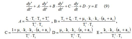
I took the formulation of the problem from [3], in it I was attracted by the variety of the structure of the object of regulation. In the course corrected several errors. So, in the final differential equation the square was lost at T2, the tables for a2 did not correspond to the results of the approximation. In addition, he introduced the control setup in the form of a single infinite impulse to liven up the image of the transition process. It is somehow not natural for the PID controller, it looks in [3].
We will explore the regulatory system with the following structural scheme.

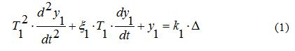
- Oscillatory link [4] is described by a differential equation of the second order.
- Linear static link, determining the dependence of the output on the input of which is determined by tabular data. Data can be obtained experimentally. Due to the inaccuracies in the data removal, linear approximation should be applied.
 .
. - The second linear static link - the dependence of the output on the input is determined by tabular data, which can be obtained experimentally. Due to the errors in the data being removed, a linear approximation should be applied
 .
. - Linear dynamic link, the input of which receives the sum of signals from blocks 2,3

The link has a transfer function, which is described by a linear differential equation of the first order.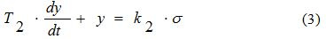
- PID controller with a known regulation law, in which the proportionality factor is used to tune the object of regulation
 with linear function, the coefficient of differentiation
  with the first derivative and the integration coefficient
  with indefinite integral.
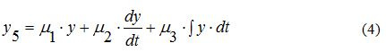
A single input action 1 (t) is converted into an operator form as 1 / p . We translate into an operator form of the equation 1.4 as a result we get.
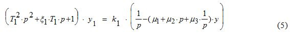
Differentiate both sides of (5), for this we simply multiply by the operator p, we get.

We translate equation (2), (3) into an operator form and express y (y1).
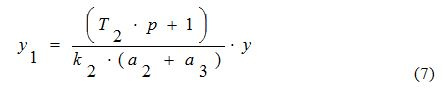
Substitute (7) in (6) we get:

Let us move (8) into the time domain; for this, we replace the operator form with a differential equation.
Solving the problem of determining the PID controller settings in Python
Set the following parameters of the control object:
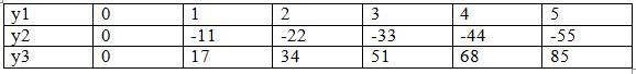
T1 = 7.0; T2 = 5.0; s = 0.4; k1 = 5.5; k2 = 5.5. The data for the approximation of the characteristics of links 2,3 are summarized in the table.
Let us set aside an object without a regulator, for this we accept
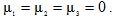 .
.Program code
#!/usr/bin/python # -*- coding: utf-8 -*- import numpy as np from scipy.integrate import odeint import matplotlib.pyplot as plt def mnkLIN(x,y,q): # a=round((len(x)*sum([x[i]*y[i] for i in range(0,len(x))])-sum(x)*sum(y))/(len(x)*sum([x[i]**2 for i in range(0,len(x))])-sum(x)**2),3) b=round((sum(y)-a*sum(x))/len(x) ,3) y1=[round(a*w+b ,3) for w in x] s=[round((y1[i]-y[i])**2,3) for i in range(0,len(x))] sko=round((sum(s)/(len(x)-1))**0.5,3) if q==1: plt.subplot(221) plt.plot(x, y, color='r', linewidth=2, marker='o', label=' a= %s'%str(a)) plt.plot(x, y1, color='g', linestyle=' ', marker='o', label=' =%s'%str(sko)) plt.legend(loc='best') plt.grid(True) else: plt.subplot(222) plt.plot(x, y, color='r', linewidth=2, marker='o', label=' a= %s'%str(a)) plt.plot(x, y1, color='g', linestyle=' ', marker='o', label=' =%s'%str(sko)) plt.legend(loc='best') plt.grid(True) return a T1=7.0;T2=5.0;s=0.4;k1=5.5;k2=5.5# . x=[0,1,2,3,4,5] y=[0,-11,-22,-33,-44,-55] a2=mnkLIN(x,y,1) x=[0,1,2,3,4,5] y=[0,17,34,51,68,85] a3=mnkLIN(x,y,2) #m1=0.5;m2=2.0;m3=0.3# . m1=0.0;m2=0.0;m3=0.0 a=a2+a3 A=round((s*T1*T2+T1**2)/(T1*T2**2),3) B=round((T2+s*T1+k1*k2*m2*a)/(T1*T2**2),3) C=round((1+k1*k2*m1*a)/(T1*T2**2),3) D=round(k1*k2*m3*a/(T1*T2**2),3) E=round(k1*k2*a/(T1*T2**2),3) def f(y, t):# . y1,y2,y3,y4 = y return [y2,y3,y4,-A*y4-B*y3-C*y2-D*y1+E] t = np.linspace(0,100,10000) y0 = [0,1,0,0]# w = odeint(f, y0, t) y1=w[:,0] # y2=w[:,1] # plt.subplot(223) plt.plot(t,y1,linewidth=1, label=' p- %s,d- %s,i- %s,'%(str(m1),str(m2),str(m3))) plt.ylabel("z") plt.xlabel("t") plt.legend(loc='best') plt.grid(True) plt.show() Result robots program.
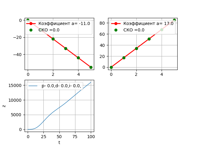
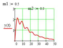
Without the PID controller, the object went to the "spacing". After preliminary selection of the PID parameters, we get.
We will change the table data for the third link, we will double a3.

The regulator is stable.
Choosing a function to solve equation (9) in Python and comparing results with a solution on Matcad
I used the odeint function from the scipy library. Integrate.
def f(y, t):# . y1,y2,y3,y4 = y return [y2,y3,y4,-A*y4-B*y3-C*y2-D*y1+E] t = np. linspace(0,100,10000) y0 = [0,1,0,0]# w = odeint(f, y0, t) y1=w[:,0] # y2=w[:,1] # If equation (9) is restructured so that the derivative on the left side is of higher order, and everything else on the right side, we get.
So the function def f (y, t) is built. The odeint function has three required arguments and looks like this odeint (func, y0, t [, args = (), ...]) .
For comparison, we derive the values of the variables A, B, C, D, E used in the above def f (y, t) function, we get 0.36 7.996 1.994 1.193 3.976. On Mathcad 14, we compose a program for solving the differential equation (9) and construct a transition characteristic.
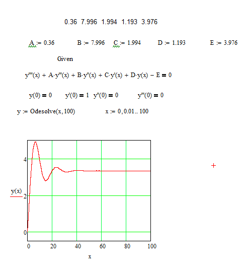
Charts and numeric values are completely identical. Thus, the Odesolve Mathcad and odeint Python functions provide the same numerical solutions to the problem presented in the article.
Conclusion
At this stage of development, the Python programming language with SciPy and NumPy libraries can be effectively used for numerical simulation of automatic control loops containing dynamic and static links.
Links
- Automated tuning of the PID controller for the control object of the tracking system using the MATLAB Simulink software package A. V. B.1, M. A.2 Kosolapov, I. A.3 Maslov, G. I. Tarasova
- PID controller tuning methods in matlab simulink.
- PID selection.
- Model of an oscillating link in the mode of resonant vibrations in Python.
Source: https://habr.com/ru/post/328608/
All Articles