Introduction to OpenCV in relation to the recognition of road marking lines
Hi, Habr! We publish graduate material from our Deep Learning program and Big Data Program Coordinator, Cyril Danyluk, about his experience of using the OpenCV computer vision framework to determine road marking lines.
Some time ago I started the program from Udacity: “Self-Driving Car Engineer Nanodegree” . It consists of many projects on various aspects of building a driving system on autopilot. I present to you my decision to the first project: a simple linear road marking detector. To understand what happened in the end, watch the video first:
')
The goal of this project is to build a simple linear model for frame-by-frame recognition of lanes: at the input we get a frame, a series of transformations, which we will discuss later, process it, we get a filtered image that can be vectorized and trained two independent linear regressions: one for each band. The project is intentionally simple: only a linear model, only good weather conditions and visibility, only two marking lines. Naturally, this is not a production-solution, but even such a project allows plenty to play with OpenCV, filters and, in general, helps to feel the difficulties that autopilot developers face in cars.
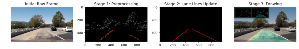
The process of building a detector consists of three basic steps:
First, a 3-channel image of the RGB format is fed to the input of the
I tried to approach the task in the OOP style (unlike most analytical tasks): so that each of the steps turned out to be isolated from the others.
The first stage of our work is well known to the data scientist and to all those who work with “raw” data: first we need to do data preprocessing, and then vectorize it into a form that is understandable for algorithms. The general pipeline for pre-processing and vectorization of the original image is as follows:
Our project uses OpenCV - one of the most popular frameworks for working with images at the pixel level using matrix operations.
First, we convert the original RGB image to HSV — it is in this color model that it is convenient to select specific color ranges (and we are interested in shades of yellow and white to determine lanes).
Pay attention to the screenshot below: it is much more difficult to select “all yellow” in RGB than in HSV.

After transferring the image to HSV, some recommend applying a Gaussian blur, but in my case it reduced the quality of recognition. The next stage is binarization (image conversion into a binary mask with colors of interest to us: shades of yellow and white).
Finally, we are ready to vectorize our image. Apply two transformations:
Obviously, the upper part of the image is unlikely to contain markup lines, so it can be ignored. There are two ways: either immediately paint the top of our binary mask with black, or think over more clever line filtering. I chose the second method: I considered that everything that is above the horizon line cannot be a marking line.
The horizon line (vanishing point) can be determined by the point at which the right and left lanes converge.
Road marking lines will be updated using the
In order to facilitate the process, I decided to use OOP and present the road marking lines as instances of the
Let's take a closer look at the
Each instance of the
Thus, to determine the belonging to the marking line, we use a rather trivial logic: we make decisions based on the slope of the line and the distance to the marking. The method is not perfect, but it worked for my simple conditions.
The
The stabilization of the obtained road marking lines is very important: the original image is very noisy, and the determination of the stripes occurs frame-by-frame. Any shadow or heterogeneity of the pavement immediately changes the color of the markup to one that our detector cannot detect ... In the process, I used several methods of stabilization:
For example, for
The stability indicator of the marking line in the current frame is described by objects of the
As a result, we get fairly stable lines:
In order for the lines to be drawn correctly, I wrote a fairly simple algorithm that calculates the coordinates of the horizon point, which we have already talked about. In my project, this point is needed for two things:
To visualize the entire strip definition process, I made a small
As can be seen from the code, I superimpose two images on the original video: one with a binary mask, the second with the lines of Hough (transformed into dots) passed through all our filters. I apply two lanes to the original video itself (linear regression over the points from the previous image). The green rectangle is an indicator of the presence of "unstable" lines: if they exist, it becomes red. The use of such an architecture makes it quite easy to change and combine frames that will be displayed as a dashboard, allowing you to simultaneously visualize many components and all this without any significant changes in the source code.
This project is still far from complete: the more I work on it, the more things that need improvement, I find:
All project source code is available on GitHub by reference .
Of course, this post should be the fun part. Let's see how miserable the detector becomes on a mountain road with frequent changes in direction and light. At first, everything seems to be normal, but in the future the error in the definition of the bands accumulates, and the detector no longer has time to monitor them:

And in the forest, where the light changes very quickly, our detector completely failed the task:

By the way, one of the following projects is to make a non-linear detector that will cope with the “forest” task. Follow new posts!
→ The original post in Medium in English .
Some time ago I started the program from Udacity: “Self-Driving Car Engineer Nanodegree” . It consists of many projects on various aspects of building a driving system on autopilot. I present to you my decision to the first project: a simple linear road marking detector. To understand what happened in the end, watch the video first:
')
The goal of this project is to build a simple linear model for frame-by-frame recognition of lanes: at the input we get a frame, a series of transformations, which we will discuss later, process it, we get a filtered image that can be vectorized and trained two independent linear regressions: one for each band. The project is intentionally simple: only a linear model, only good weather conditions and visibility, only two marking lines. Naturally, this is not a production-solution, but even such a project allows plenty to play with OpenCV, filters and, in general, helps to feel the difficulties that autopilot developers face in cars.
The principle of the detector
The process of building a detector consists of three basic steps:
- Data pre-processing, noise filtering and vectorization of the image.
- Update road marking lines from data from the first step.
- Drawing updated lines and other objects on the original image.
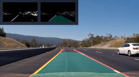
First, a 3-channel image of the RGB format is fed to the input of the
image_pipeline function, which is then filtered, converted, and the Line and Lane objects are updated inside the function. Then all the necessary elements are drawn over the image itself, as shown below:I tried to approach the task in the OOP style (unlike most analytical tasks): so that each of the steps turned out to be isolated from the others.
Step 1: Pretreatment and Vectoring
The first stage of our work is well known to the data scientist and to all those who work with “raw” data: first we need to do data preprocessing, and then vectorize it into a form that is understandable for algorithms. The general pipeline for pre-processing and vectorization of the original image is as follows:
blank_image = np.zeros_like(image) hsv_image = cv2.cvtColor(image, cv2.COLOR_RGB2HSV) binary_mask = get_lane_lines_mask(hsv_image, [WHITE_LINES, YELLOW_LINES]) masked_image = draw_binary_mask(binary_mask, hsv_image) edges_mask = canny(masked_image, 280, 360) # Correct initialization is important, we cheat only once here! if not Lane.lines_exist(): edges_mask = region_of_interest(edges_mask, ROI_VERTICES) segments = hough_line_transform(edges_mask, 1, math.pi / 180, 5, 5,Our project uses OpenCV - one of the most popular frameworks for working with images at the pixel level using matrix operations.
First, we convert the original RGB image to HSV — it is in this color model that it is convenient to select specific color ranges (and we are interested in shades of yellow and white to determine lanes).
Pay attention to the screenshot below: it is much more difficult to select “all yellow” in RGB than in HSV.
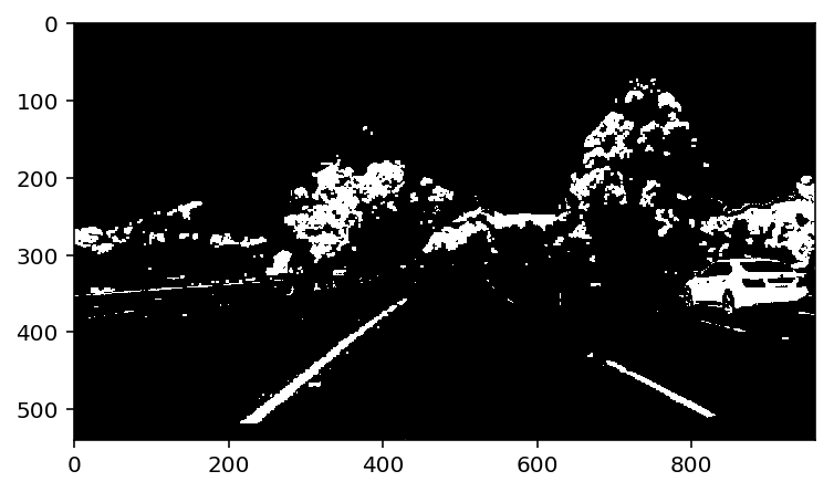
After transferring the image to HSV, some recommend applying a Gaussian blur, but in my case it reduced the quality of recognition. The next stage is binarization (image conversion into a binary mask with colors of interest to us: shades of yellow and white).
Finally, we are ready to vectorize our image. Apply two transformations:
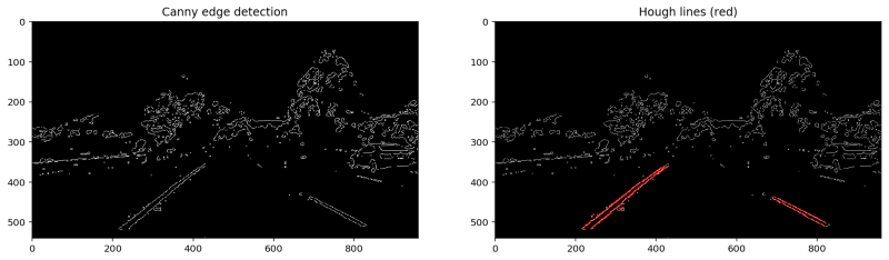
- Canny Boundary Detector : an optimal boundary detection algorithm that calculates image intensity gradients, and then removes weak boundaries using two thresholds, leaving the desired ones (we use
(280, 360)) as threshold values in thecannyfunction. - Hough Transformation: after obtaining the boundaries using the Canny algorithm, we can connect them using lines. I do not want to go into the mathematics of the algorithm - it is worthy of a separate post - this link or the link above will help you if you are interested in the method. The main thing is that by applying this transformation, we get a set of lines, each of which, after a little additional processing and filtering, becomes an instance of the Line class with a known angle of inclination and a free member.
Obviously, the upper part of the image is unlikely to contain markup lines, so it can be ignored. There are two ways: either immediately paint the top of our binary mask with black, or think over more clever line filtering. I chose the second method: I considered that everything that is above the horizon line cannot be a marking line.
The horizon line (vanishing point) can be determined by the point at which the right and left lanes converge.
Step 2: Update Road Marking Lines
Road marking lines will be updated using the
update_lane(segments) function in image_pipeline , which at the input receives segments objects from the last step (which are actually Line objects from the Hough transformation).In order to facilitate the process, I decided to use OOP and present the road marking lines as instances of the
Lane class: Lane.left_line, Lane.right_line . Some students limited themselves to adding the `lane` object to global namespace, but I'm not a fan of global variables in code.Let's take a closer look at the
Lane and Line classes and their instances:Each instance of the
Line class is a separate line: a road marking piece or just any line that will be defined by the Hough Transform, while the main purpose of Lane objects is to identify whether this line is a road marking segment. To do this, we will be guided by the following logic:- The line can not be horizontal and should have a moderate slope.
- The difference between the slopes of the road marking line and the candidate line cannot be too high.
- The candidate line must not be far from the road marking to which it belongs.
- Candidate line should be below the horizon
Thus, to determine the belonging to the marking line, we use a rather trivial logic: we make decisions based on the slope of the line and the distance to the marking. The method is not perfect, but it worked for my simple conditions.
The
Lane class is a container for the left and right marking lines (refactoring just asks). The class also presents several methods related to working with markup lines, the most important of which is fit_lane_line . In order to create a new markup line, I represent suitable markup segments as points, and then I approximate them with a first-order polynomial (that is, a line) using the usual numpy.polyfit functionThe stabilization of the obtained road marking lines is very important: the original image is very noisy, and the determination of the stripes occurs frame-by-frame. Any shadow or heterogeneity of the pavement immediately changes the color of the markup to one that our detector cannot detect ... In the process, I used several methods of stabilization:
- Buffers The resulting marking line stores the N previous states and successively adds the state of the marking line on the current frame to the buffer.
- Additional line filtering taking into account data in the buffer. If, after transformation and cleaning, we could not get rid of the noise in the data, then there is a possibility that our line will be an outlier, and, as we know, the linear model is sensitive to outliers. Therefore, for us, the fundamentally high value of accuracy is even at the expense of a significant loss of completeness. Simply put, it is better to filter the correct line than to add an outlier to the model. Especially for such cases, I created a
DECISION_MAT— a “decision maker” matrix that decides how to relate the current slope of the line to the average of all the lines in the buffer.
For example, for
DECISION_MAT = [ [ 0.1, 0.9] , [1, 0] ] we consider the choice of two solutions: to consider the line unstable (ie, a potential outlier), or stable (its slope corresponds to the average slope of the lines of this band in the buffer plus / minus threshold). If the line is unstable, we still want not to lose it: it can carry information about the real turn of the road. We will simply take it into account with a small coefficient (in this case, 0.1). For a stable line, we will simply use its current parameters without any weighting from previous data.The stability indicator of the marking line in the current frame is described by objects of the
Lane class: Lane.right_lane.stable and Lane.left_lane.stable , which are Boolean. If at least one of these variables is set to False , I render it as a red polygon between two lines (below you can see how it looks).As a result, we get fairly stable lines:
Step 3: Draw and update the original image
In order for the lines to be drawn correctly, I wrote a fairly simple algorithm that calculates the coordinates of the horizon point, which we have already talked about. In my project, this point is needed for two things:
- Limit the extrapolation of marking lines to this point.
- Filter all Hough lines above the horizon.
To visualize the entire strip definition process, I made a small
image augmentation : def draw_some_object(what_to_draw, background_image_to_draw_on, **kwargs): # do_stuff_and_return_image # Snapshot 1 out_snap1 = np.zeros_like(image) out_snap1 = draw_binary_mask(binary_mask, out_snap1) out_snap2 = draw_filtered_lines(segments, out_snap1) snapshot1 = cv2.resize(deepcopy(out_snap1), (240,135)) # Snapshot 2 out_snap2 = np.zeros_like(image) out_snap2 = draw_canny_edges(edges_mask, out_snap2) out_snap2 = draw_points(Lane.left_line.points, out_snap2, Lane.COLORS['left_line']) out_snap2 = draw_points(Lane.right_line.points, out_snap2, Lane.COLORS['right_line']) out_snap2 = draw_lane_polygon(out_snap2) snapshot2 = cv2.resize(deepcopy(out_snap2), (240,135)) # Augmented image output = deepcopy(image) output = draw_lane_lines([Lane.left_line, Lane.right_line], output, shade_background=True) output = draw_lane_polygon(output) output = draw_dashboard(output, snapshot1, snapshot2) return outputAs can be seen from the code, I superimpose two images on the original video: one with a binary mask, the second with the lines of Hough (transformed into dots) passed through all our filters. I apply two lanes to the original video itself (linear regression over the points from the previous image). The green rectangle is an indicator of the presence of "unstable" lines: if they exist, it becomes red. The use of such an architecture makes it quite easy to change and combine frames that will be displayed as a dashboard, allowing you to simultaneously visualize many components and all this without any significant changes in the source code.
What's next?
This project is still far from complete: the more I work on it, the more things that need improvement, I find:
- To make the detector nonlinear so that it can work successfully, for example, in the mountains, where turns are at every turn.
- Make a projection of the road as a “top view” - this will greatly simplify the definition of lanes.
- Recognition of the road. It would be great to recognize not only the markup, but also the road itself, which will greatly facilitate the work of the detector.
All project source code is available on GitHub by reference .
PS And now we break everything!
Of course, this post should be the fun part. Let's see how miserable the detector becomes on a mountain road with frequent changes in direction and light. At first, everything seems to be normal, but in the future the error in the definition of the bands accumulates, and the detector no longer has time to monitor them:
And in the forest, where the light changes very quickly, our detector completely failed the task:
By the way, one of the following projects is to make a non-linear detector that will cope with the “forest” task. Follow new posts!
→ The original post in Medium in English .
Source: https://habr.com/ru/post/328422/
All Articles