Metrics in machine learning tasks
Hi, Habr!

In problems of machine learning, metrics are used to assess the quality of models and compare various algorithms, and their selection and analysis is an indispensable part of the work of a datasanist.
In this article, we will look at some of the quality criteria in classification problems, discuss what is important when choosing a metric, and what can go wrong.
Metrics in classification problems
To demonstrate the useful functions of sklearn and a visual presentation of metrics, we will use dataset for outflow of clients by the telecom operator.
import pandas as pd import matplotlib.pyplot as plt from matplotlib.pylab import rc, plot import seaborn as sns from sklearn.preprocessing import LabelEncoder, OneHotEncoder from sklearn.model_selection import cross_val_score from sklearn.linear_model import LogisticRegression from sklearn.ensemble import RandomForestClassifier, GradientBoostingClassifier from sklearn.metrics import precision_recall_curve, classification_report from sklearn.model_selection import train_test_split df = pd.read_csv('../../data/telecom_churn.csv') df.head(5) 
# # dummy- ( , ) d = {'Yes' : 1, 'No' : 0} df['International plan'] = df['International plan'].map(d) df['Voice mail plan'] = df['Voice mail plan'].map(d) df['Churn'] = df['Churn'].astype('int64') le = LabelEncoder() df['State'] = le.fit_transform(df['State']) ohe = OneHotEncoder(sparse=False) encoded_state = ohe.fit_transform(df['State'].values.reshape(-1, 1)) tmp = pd.DataFrame(encoded_state, columns=['state ' + str(i) for i in range(encoded_state.shape[1])]) df = pd.concat([df, tmp], axis=1) Accuracy, precision and recall
Before moving on to the metrics themselves, it is necessary to introduce an important concept for describing these metrics in terms of classification errors - the confusion matrix .
Suppose that we have two classes and an algorithm that predicts that each object belongs to one of the classes, then the classification error matrix will look like this:
| True Positive (TP) | False Positive (FP) | |
| False Negative (FN) | True Negative (TN) |
Here - is the answer of the algorithm on the object, and - true class label on this object.
Thus, classification errors are of two types: False Negative (FN) and False Positive (FP).
X = df.drop('Churn', axis=1) y = df['Churn'] # train test, X_train, X_test, y_train, y_test = train_test_split(X, y, stratify=y, test_size=0.33, random_state=42) # lr = LogisticRegression(random_state=42) lr.fit(X_train, y_train) # sklearn def plot_confusion_matrix(cm, classes, normalize=False, title='Confusion matrix', cmap=plt.cm.Blues): """ This function prints and plots the confusion matrix. Normalization can be applied by setting `normalize=True`. """ plt.imshow(cm, interpolation='nearest', cmap=cmap) plt.title(title) plt.colorbar() tick_marks = np.arange(len(classes)) plt.xticks(tick_marks, classes, rotation=45) plt.yticks(tick_marks, classes) if normalize: cm = cm.astype('float') / cm.sum(axis=1)[:, np.newaxis] print("Normalized confusion matrix") else: print('Confusion matrix, without normalization') print(cm) thresh = cm.max() / 2. for i, j in itertools.product(range(cm.shape[0]), range(cm.shape[1])): plt.text(j, i, cm[i, j], horizontalalignment="center", color="white" if cm[i, j] > thresh else "black") plt.tight_layout() plt.ylabel('True label') plt.xlabel('Predicted label') font = {'size' : 15} plt.rc('font', **font) cnf_matrix = confusion_matrix(y_test, lr.predict(X_test)) plt.figure(figsize=(10, 8)) plot_confusion_matrix(cnf_matrix, classes=['Non-churned', 'Churned'], title='Confusion matrix') plt.savefig("conf_matrix.png") plt.show() 
Accuracy
An intuitive, obvious and almost unused metric is accuracy - the proportion of correct answers of the algorithm:
This metric is useless in problems with unequal classes, and this is easy to show with an example.
Suppose we want to evaluate the work of spam mail filter. We have 100 non-spam emails, 90 of which our classifier defined correctly (True Negative = 90, False Positive = 10), and 10 spam letters, 5 of which the classifier also determined correctly (True Positive = 5, False Negative = five).
Then accuracy:
However, if we simply predict all letters as non-spam, we will get higher accuracy:
At the same time, our model does not have any predictive power at all, since initially we wanted to identify spam letters. To overcome this we will be helped by the transition from the metrics common to all classes to the individual indicators of the quality of the classes.
Precision, recall and F-measure
To assess the quality of the algorithm’s work on each of the classes separately, we introduce precision (accuracy) and recall (complete) metrics.
Precision can be interpreted as the proportion of objects that the classifier calls positive and at the same time truly positive, and the recall shows what proportion of objects of the positive class from all objects of the positive class the algorithm has found.

Precisely, the introduction of precision does not allow us to write all the objects into one class, since in this case we get an increase in the False Positive level. Recall demonstrates the ability of an algorithm to detect a given class in general, and precision an ability to distinguish this class from other classes.
As we noted earlier, classification errors are of two types: False Positive and False Negative. In statistics, the first type of error is called the error of the first kind, and the second - the error of the second kind. In our task of determining the outflow of subscribers, the mistake of the first kind will be the acceptance of the loyal subscriber for the outgoing, since our null hypothesis is that none of the subscribers leaves, and we reject this hypothesis. Accordingly, an error of the second kind will be the “omission” of the outgoing subscriber and the erroneous acceptance of the null hypothesis.
Precision and recall do not depend, as opposed to accuracy, on the class ratios and are therefore applicable in conditions of unbalanced samples.
Often, in actual practice, the challenge is to find the optimal (for the customer) balance between these two metrics. A classic example is the problem of determining customer churn.
Obviously, we cannot find all the customers leaving for the outflow and only them. But, having defined a strategy and a resource for retaining customers, we can choose the necessary thresholds for precision and recall. For example, you can focus on retaining only highly profitable customers or those who are more likely to leave, since we are limited in call center resources.
Usually, when optimizing the hyperparameters of the algorithm (for example, in the case of iteration over the GridSearchCV grid), one metric is used, the improvement of which we expect to see on the test set.
There are several different ways to combine precision and recall into an aggregated quality criterion. F-measure (in general ) - harmonic precision and recall:
in this case, determines the weight of accuracy in the metric, and is the harmonic mean (with a factor of 2, so that in the case of precision = 1 and recall = 1 )
The F-measure reaches a maximum with completeness and accuracy equal to one, and is close to zero if one of the arguments is close to zero.
In sklearn, there is a convenient _metrics.classification report function that returns recall, precision and F-measure for each of the classes, as well as the number of instances of each class.
report = classification_report(y_test, lr.predict(X_test), target_names=['Non-churned', 'Churned']) print(report) | class | precision | recall | f1-score | support |
|---|---|---|---|---|
| Non-churned | 0.88 | 0.97 | 0.93 | 941 |
| Churned | 0.60 | 0.25 | 0.35 | 159 |
| avg / total | 0.84 | 0.87 | 0.84 | 1100 |
It should be noted here that in the case of tasks with unbalanced classes that prevail in actual practice, it is often necessary to resort to techniques of artificially modifying dataset to equalize the ratio of classes. There are many of them, and we will not touch them; here you can look at some of the methods and choose the right one for your task.
AUC-ROC and AUC-PR
When converting the real answer of the algorithm (as a rule, the probability of belonging to a class, see separately SVM ) into a binary label, we must choose a threshold at which 0 becomes 1. The threshold of 0.5 seems natural and close, but it is not always turns out to be optimal, for example, with the aforementioned unbalance of classes.
One way to evaluate the model as a whole, without being tied to a specific threshold, is the AUC-ROC (or ROC AUC) - area ( A rea U nder C urve) under the error curve ( R eceiver O perating C haracteristic curve). This curve is a line from (0,0) to (1,1) in the coordinates of True Positive Rate (TPR) and False Positive Rate (FPR):
TPR is already known to us, this is completeness, and the FPR shows what proportion of negative objects of the class the algorithm predicted incorrectly. In the ideal case, when the classifier does not make mistakes (FPR = 0, TPR = 1) we get the area under the curve equal to one; otherwise, when the classifier randomly gives out the class probabilities, AUC-ROC will tend to 0.5, since the classifier will produce the same amount of TP and FP.
Each point on the graph corresponds to the choice of a certain threshold. The area under the curve in this case shows the quality of the algorithm (more - better), besides this, the steepness of the curve itself is important - we want to maximize TPR while minimizing FPR, which means that our curve should ideally go to the point (0,1).
sns.set(font_scale=1.5) sns.set_color_codes("muted") plt.figure(figsize=(10, 8)) fpr, tpr, thresholds = roc_curve(y_test, lr.predict_proba(X_test)[:,1], pos_label=1) lw = 2 plt.plot(fpr, tpr, lw=lw, label='ROC curve ') plt.plot([0, 1], [0, 1]) plt.xlim([0.0, 1.0]) plt.ylim([0.0, 1.05]) plt.xlabel('False Positive Rate') plt.ylabel('True Positive Rate') plt.title('ROC curve') plt.savefig("ROC.png") plt.show() 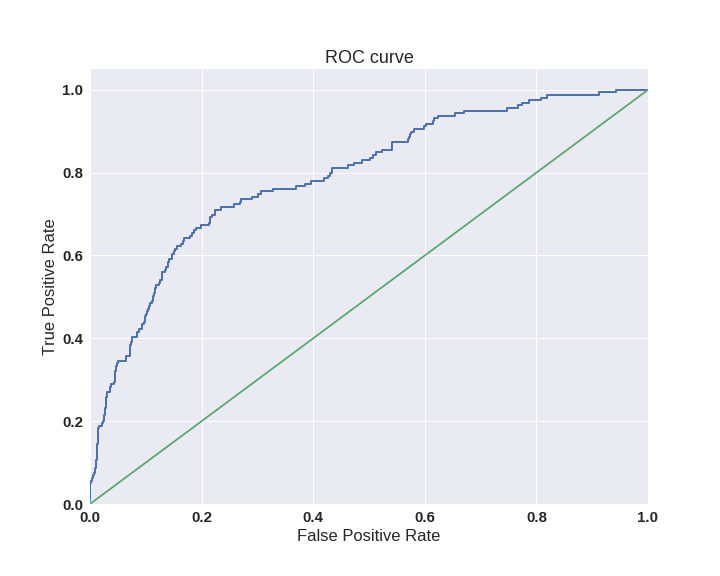
The AUC-ROC criterion is resistant to unbalanced classes (spoiler: alas, not so simple) and can be interpreted as the probability that a randomly selected positive object will be ranked higher by the classifier (will have a higher probability of being positive) than a randomly selected negative object .
Consider the following task: we need to select 100 relevant documents from 1 million documents. We have mastered two algorithms:
- Algorithm 1 returns 100 documents, 90 of which are relevant. In this way,
- Algorithm 2 returns 2000 documents, 90 of which are relevant. In this way,
Most likely, we would choose the first algorithm that gives out very little False Positive against the background of its competitor. But the difference in the False Positive Rate between these two algorithms is extremely small - only 0.0019. This is a consequence of the fact that AUC-ROC measures the proportion of False Positive relative to True Negative and in tasks where the second (larger) class is not so important for us may not give an entirely adequate picture when comparing algorithms.
In order to improve the situation, back to the completeness and accuracy:
- Algorithm 1
- Algorithm 2
There is already a significant difference between the two algorithms - 0.855 exactly!
Precision and recall are also used to create a curve and, similarly to the AUC-ROC, find the area under it.

It can be noted here that on small datasets, the area under the PR curve may be overly optimistic, because it is calculated using the trapezoid method, but usually in such problems there is enough data. For details on the relationship between AUC-ROC and AUC-PR, please contact here .
Logistic loss
The logistic loss function, defined as:
here - this is the algorithm's answer to th object - true class mark on th object, and sample size.
Details about the mathematical interpretation of the logistic loss function have already been written in the post about linear models.
This metric does not often appear in business requirements, but often in tasks on kaggle .
Intuitively, minimizing logloss can be presented as a task of maximizing accuracy by a penalty for incorrect predictions. However, it should be noted that logloss is heavily penalized for the confidence of the classifier in the wrong answer.
Consider an example:
def logloss_crutch(y_true, y_pred, eps=1e-15): return - (y_true * np.log(y_pred) + (1 - y_true) * np.log(1 - y_pred)) print('Logloss %f' % logloss_crutch(1, 0.5)) >> Logloss 0.693147 print('Logloss %f' % logloss_crutch(1, 0.9)) >> Logloss 0.105361 print('Logloss %f' % logloss_crutch(1, 0.1)) >> Logloss 2.302585 Note how logloss has grown dramatically with the wrong answer and confident classification!
Therefore, an error on one object can give a significant deterioration in the total error on the sample. Such objects are often emissions that need to be remembered to filter or be considered separately.
Everything falls into place if you draw a logloss graph:

It can be seen that the closer to zero the response of the algorithm with ground truth = 1, the higher the error value and the steeper the curve grows.
Summing up:
- In the case of a multi-class classification, you need to carefully monitor the metrics of each class and follow the logic of solving the problem , rather than optimizing the metric
- In case of unequal classes, it is necessary to select the balance of classes for training and a metric that will correctly reflect the quality of classification.
- The choice of a metric should be done with a focus on the subject area, pre-processing the data and, possibly, segmenting (as is the case with the division into rich and poor clients)
useful links
- The course of Evgeny Sokolov: Seminar on the choice of models (there is information on the metrics of regression problems)
- Problems on AUC-ROC from A.G. Dyakonova
- You can also read about other metrics on kaggle . For each metric description added link to the competition, where it was used
- Presentation of Bogdan Melnik aka ld86 about training on unbalanced samples
Thanks
Thank you mephistopheies and madrugado for help in preparing the article.
')
Source: https://habr.com/ru/post/328372/
All Articles