Applied application of the nonlinear programming problem
Good day, Habr! At one time, as a junior student, I began to engage in research work in the field of the theory of optimization and synthesis of optimal nonlinear dynamic systems. Around the same time, there was a desire to popularize this area, to share their experiences and thoughts with people. This is confirmed by a couple of my childhood immature articles on Habré. However, at that time, this idea was daunting for me. Perhaps because of my employment, inexperience, inability to work with criticism and advice, or something else. You can endlessly try to find the cause, but this will not change the situation: I threw this idea on the shelf, where it lay safely and gathering dust until that moment.
Having finished the specialty and preparing for the defense of my Ph.D. thesis, I asked myself quite a logical question: “What next?” Having experience in both regular work and research, I returned to the very idea that it would seem like it had to drown under a layer of dust. But I returned to this idea in a more conscious form.
I decided to start developing software related to the industry I have been engaged in for 8 years and my personal academic predilections, which include optimization methods and machine learning.
')

Well, all who are interested:
Being engaged in the implementation of software for my diploma (and later the thesis), I approached this issue “head on”: I did not care how flexible the system would be, how easy it would be to modify. The desire to get results here and now, along with inexperience, led to the fact that the code constantly had to be rewritten, which, of course, had no positive effect on professional development. Already, I understand that, no matter how desirable, it is impossible to rush headlong to solve the problem. It is necessary to penetrate into its essence, evaluate the existing knowledge, understand what is missing, compare the concepts of the domain to classes, interfaces and abstractions. In short, you need to realize the existing reserves and correctly approach the design of the software architecture.
As you may have guessed, this article will be devoted to the development and description of the first elements of the future application.
Habré has a large number of articles on software development methodologies. For example, in this quite clearly described the main approaches. Let us dwell on each of them:
I will try to stick to the concepts of the Agile model. At each iteration of the development, a specific set of goals and objectives will be offered, which will be covered in more detail in the articles.
So, at the moment there is the following formulation of a common task: the software being developed must implement various optimization algorithms (like classical analytical, as well as modern heuristic) and machine learning (classification algorithms, clustering, reduction of space dimension, regression). The final final goal is to develop methods for applying these algorithms in the field of optimal control synthesis and creating trading strategies in financial markets. Scala was chosen as the main language for development.
So, in this work I will tell:
Due to the fact that I have devoted most of my research practice to solving optimization problems, it will be more convenient for me to operate from this point of view.
Usually, a solution to an optimization problem, no matter how trite and tongue-tied it may sound, is the search for some “optimal” (in terms of task conditions) object. The concepts of “optimality” vary from one subject area to another. For example, in the task of finding the minimum of a function, it is required to find the point to which the smallest value of the objective function corresponds. In the meta-optimization task, it is necessary to determine the parameters of the algorithm at which it gives the most accurate result / most quickly work out / gives the most stable result, in the problem of optimal control synthesis it is required to synthesize the controller, which allows to transfer the object to the terminal state in the shortest time, etc. I am sure that every specialist will be able to continue this list of tasks related to his professional sphere.
In mathematics, special attention is paid to the problem of nonlinear programming , to which a large number of other applied problems can be reduced. In general, for the formulation of a nonlinear programming problem, it is required to specify
Thus, the essence of this task can be described as follows: it is required to find a vector in the search area that provides the minimum / maximum value of the objective function.
There is a huge number of algorithms for solving this problem. Conventionally, they can be divided into two groups:
In principle, heuristic algorithms can be perceived as a method of directional searching. In this group you can find well-known genetic algorithms , annealing simulation algorithm , various population algorithms. A large number of algorithms is explained quite simply: there is no universal algorithm that would be good at the same time for all types of tasks. Someone copes better with convex functions, the other is aimed at working with functions that have a ravine structure of level lines, the third specializes in multi-extremal functions. As in life - everything has its own specialization.
Based on the above reasoning, it seems to me that the easiest way to work with two concepts: transformation and algorithm . On them and dwell.
Due to the fact that almost any procedure / function / algorithm can be considered as a certain transformation, we will operate with this object as one of the basic ones.
The following hierarchy between different types of transformations is proposed:

Let us dwell on the elements in more detail:
The given abstractions, at first glance, cover the main types of transformations that may be needed for further formulation of the tasks.
I think it will be natural to define an algorithm as a set of three operations: initialization, iterative part and termination. To the input of the algorithm is given some task (Task) . During initialization, the generation of the initial state (State) of the algorithm occurs, which is modified during the repetition of the iterative part. At the end, using the termination procedure from the last state of the algorithm, an object is created corresponding to the type R of the output parameter of the algorithm.
Thus, to create a specific algorithm, it will be necessary to override the three previously described procedures.
Well, the first two points of the promised program are covered, it's time to move on to the third.
Both algorithms are well described in various sources, so I think that readers will not be difficult to deal with them. Instead, I will draw parallels to the abstractions described earlier.
A clusterizer built using the K-Means algorithm is uniquely determined by its centroids. The K-Means algorithm itself is a constant replacement of the current centroids with new centroids, calculated as the average of all vectors in individual clusters. Thus, at any time, the state of the K-Means algorithm can be represented as a set of vectors.
Thus, the clusteriser can be built either directly using the K-Means algorithm, or by solving the problem of finding the optimal clusteriser, which ensures the minimum total distance of the cluster points from the corresponding centroids.
Generate several synthetic datasets of dimension 2, 3, and 5.
And "run them" through both algorithms building a cluster. The results obtained are summarized in the table:
The table shows that even a simple optimization algorithm can successfully solve the problem of constructing a simple clusterizer. At the same time, the created clusterizer will be optimal (and to be honest, suboptimal, since the optimization method used does not guarantee finding the global optimum point) in terms of the quality metric used. Naturally, the optimization algorithm used for problems of a higher dimension is hardly suitable (here it is better to use more complex and efficient algorithms based on several heuristics of different levels). For a small synthetic task, Random Search did quite well.
I would like to thank everyone who read the article, unsubscribed in the comments. In short, everyone who contributed to the creation of this work. Probably, it should be immediately noted that articles on this subject will appear as far as possible and my current workload. But I would like to say that this time I will try to bring the matter begun by me to the end.
References and literature
Having finished the specialty and preparing for the defense of my Ph.D. thesis, I asked myself quite a logical question: “What next?” Having experience in both regular work and research, I returned to the very idea that it would seem like it had to drown under a layer of dust. But I returned to this idea in a more conscious form.
I decided to start developing software related to the industry I have been engaged in for 8 years and my personal academic predilections, which include optimization methods and machine learning.
')
Well, all who are interested:
Being engaged in the implementation of software for my diploma (and later the thesis), I approached this issue “head on”: I did not care how flexible the system would be, how easy it would be to modify. The desire to get results here and now, along with inexperience, led to the fact that the code constantly had to be rewritten, which, of course, had no positive effect on professional development. Already, I understand that, no matter how desirable, it is impossible to rush headlong to solve the problem. It is necessary to penetrate into its essence, evaluate the existing knowledge, understand what is missing, compare the concepts of the domain to classes, interfaces and abstractions. In short, you need to realize the existing reserves and correctly approach the design of the software architecture.
As you may have guessed, this article will be devoted to the development and description of the first elements of the future application.
Definition of the approach to development and formulation of the main task
Habré has a large number of articles on software development methodologies. For example, in this quite clearly described the main approaches. Let us dwell on each of them:
- “Waterfall Model” - does not fit because at least of the fact that I have no clearly defined requirements, there is only a set of ideas, between which we will have to subsequently establish interaction,
- "V-Model" - not suitable for the same reason
- “Incremental Model” is a more suitable model compared to the previous ones, however, detailed formalization is also required here.
- "RAD Model" - a model that is more suitable for a team of experienced professionals,
- "Agile Model" - perfectly fits the criterion of the absence of the need to specify requirements, as well as flexibility in the development process,
- “Iterative Model” - despite the fact that the work indicates the need for clear definition of goals, ideologically such a model seems close (taking into account the words “The main task should be defined, but implementation details can evolve over time”),
- "Spiral Model" - aimed for the implementation of large projects, which can hardly be attributed to the intended software.
I will try to stick to the concepts of the Agile model. At each iteration of the development, a specific set of goals and objectives will be offered, which will be covered in more detail in the articles.
So, at the moment there is the following formulation of a common task: the software being developed must implement various optimization algorithms (like classical analytical, as well as modern heuristic) and machine learning (classification algorithms, clustering, reduction of space dimension, regression). The final final goal is to develop methods for applying these algorithms in the field of optimal control synthesis and creating trading strategies in financial markets. Scala was chosen as the main language for development.
So, in this work I will tell:
- About the optimization problem and the reasons for its choice as a fundamental object of study,
- About the main abstractions and their implementations that will allow you to use an approach based on solving applied problems by reducing them to an optimization problem,
- About the K-Means algorithm, the simplest Random Search algorithm and how to make them friends and work for the benefit of a single goal.
Optimization
Due to the fact that I have devoted most of my research practice to solving optimization problems, it will be more convenient for me to operate from this point of view.
Usually, a solution to an optimization problem, no matter how trite and tongue-tied it may sound, is the search for some “optimal” (in terms of task conditions) object. The concepts of “optimality” vary from one subject area to another. For example, in the task of finding the minimum of a function, it is required to find the point to which the smallest value of the objective function corresponds. In the meta-optimization task, it is necessary to determine the parameters of the algorithm at which it gives the most accurate result / most quickly work out / gives the most stable result, in the problem of optimal control synthesis it is required to synthesize the controller, which allows to transfer the object to the terminal state in the shortest time, etc. I am sure that every specialist will be able to continue this list of tasks related to his professional sphere.
In mathematics, special attention is paid to the problem of nonlinear programming , to which a large number of other applied problems can be reduced. In general, for the formulation of a nonlinear programming problem, it is required to specify
- arbitrary function (it fulfills the role of some quality criterion: for minimization problems, it is required to find a vector that corresponds to the smallest value, for maximization, vice versa)
- a set of constraints that essentially define the range of valid values of argument optimized function.
Thus, the essence of this task can be described as follows: it is required to find a vector in the search area that provides the minimum / maximum value of the objective function.
There is a huge number of algorithms for solving this problem. Conventionally, they can be divided into two groups:
- analytical algorithms:
- have a narrower range of tasks due to the fact that they can impose restrictions on the components of the problem,
- can enter higher level objects into the task (for example, derivatives of a certain order),
- The undoubted advantage of such methods is that for the most part they allow to obtain the result of a certain accuracy.
- heuristic algorithms:
- there is no property of guaranteed calculations, i.e. one cannot be sure that the solution obtained has fallen at least into the region of attraction of a local extremum ,
- they have less computational complexity, which makes it possible to use them in order to obtain a practically acceptable result in a reasonable time (for example, on large-scale problems, when it may take a day to receive a response using an analytical algorithm).
In principle, heuristic algorithms can be perceived as a method of directional searching. In this group you can find well-known genetic algorithms , annealing simulation algorithm , various population algorithms. A large number of algorithms is explained quite simply: there is no universal algorithm that would be good at the same time for all types of tasks. Someone copes better with convex functions, the other is aimed at working with functions that have a ravine structure of level lines, the third specializes in multi-extremal functions. As in life - everything has its own specialization.
Used abstractions
Based on the above reasoning, it seems to me that the easiest way to work with two concepts: transformation and algorithm . On them and dwell.
Transformations
Due to the fact that almost any procedure / function / algorithm can be considered as a certain transformation, we will operate with this object as one of the basic ones.
The following hierarchy between different types of transformations is proposed:
Let us dwell on the elements in more detail:
- Nonhomogeneous transformation (Inhomogeneous Transformation) - the most common type of transformation, when the classes of the input and output objects may be different
- Homogeneous Transformation - a particular type of inhomogeneous transformation, when the classes of the input and output objects are the same,
- A vector function (Vector Function) is a transformation that transforms a vector consisting of elements of set A into another vector consisting of elements of the same set,
- Function (Function) is similar to a vector function (except that the output element is now a scalar),
- Metric (Metric) - some estimating conversion that assigns a numeric value to the object.
Heterogeneous Transform Class Code
It can be seen that it contains only two methods, one of which implements the procedure for composing the composition of several transformations (only in a not quite usual order). This will be needed later to create more complex transformations from simple ones.
class InhomogeneousTransformation[A, B](transform: A => B) extends Serializable { def apply(a: A): B = transform(a) def *[C](f: InhomogeneousTransformation[B, C]) = new InhomogeneousTransformation[A, C](x => f(transform(x))) } It can be seen that it contains only two methods, one of which implements the procedure for composing the composition of several transformations (only in a not quite usual order). This will be needed later to create more complex transformations from simple ones.
Homogeneous transform class code
Here, the two type parameters were collapsed into one.
class HomogeneousTransformation[A](transform: A => A) extends InhomogeneousTransformation[A, A](transform) { } Here, the two type parameters were collapsed into one.
Class code of a vector function
There is a modified parametrization of the generalized class. Now this parameter determines what objects of which class the converted vector will consist of. Note the restriction imposed on the class, which is determined by the given code "[A <: Algebra [A]]". The restriction is expressed in the following: the objects from which the vector is composed must support the basic arithmetic operations and can be used as an argument of the usual elementary functions (exponential, trigonometric, etc.). Detailed code can be viewed on the source code, which are posted on github'e (link will be at the end of the work).
class VectorFunction[A <: Algebra[A]] (transform: Vector[A] => Vector[A])(implicit converter: Double => A) extends HomogeneousTransformation[Vector[A]](transform) { } There is a modified parametrization of the generalized class. Now this parameter determines what objects of which class the converted vector will consist of. Note the restriction imposed on the class, which is determined by the given code "[A <: Algebra [A]]". The restriction is expressed in the following: the objects from which the vector is composed must support the basic arithmetic operations and can be used as an argument of the usual elementary functions (exponential, trigonometric, etc.). Detailed code can be viewed on the source code, which are posted on github'e (link will be at the end of the work).
Codes of the Function class and the method of its implicit coercion to non-uniform transformation
class Function[A <: Algebra[A]] (transform: Vector[A] => A)(implicit converter: Double => A) extends VectorFunction[A](x => Vector("result" -> transform(x))) { def calculate(v: Vector[A]): A = transform(v) } object Function { implicit def createFromInhomogeneousTransformation[A <: Algebra[A]] (transformation: InhomogeneousTransformation[Vector[A], A])(implicit converter: Double => A) = new Function[A](x => transformation(x)) } Metric class code and related conversions
class Metric[A](transform: A => Real) extends InhomogeneousTransformation[A, Real](transform) { } object Metric { implicit def createFromInhomogeneousTransformation[A](transformation: InhomogeneousTransformation[A, Real]) = new Metric[A](x => transformation(x)) implicit def toFunction (metric: Metric[Vector[Real]])(implicit converter: Double => Real): Function[Real] = new Function[Real](x => metric(x)) } The given abstractions, at first glance, cover the main types of transformations that may be needed for further formulation of the tasks.
Algorithm
I think it will be natural to define an algorithm as a set of three operations: initialization, iterative part and termination. To the input of the algorithm is given some task (Task) . During initialization, the generation of the initial state (State) of the algorithm occurs, which is modified during the repetition of the iterative part. At the end, using the termination procedure from the last state of the algorithm, an object is created corresponding to the type R of the output parameter of the algorithm.
Class Code Algorithm
trait GeneralAlgorithm[T <: GeneralTask, S <: GeneralState, R] { def initializeRandomly(task: T): S def initializeFromSeed(task: T, seed: S): S final def initialize(task: T, state: Option[S]): S = { state match { case None => initializeRandomly(task) case Some(seed) => initializeFromSeed(task, seed) } } def iterate(task: T, state: S): S def terminate(task: T, state: S): R def prepareFolder(log: Option[String]): Unit = { if (log.isDefined) { val temp = new File(log.get) if (!temp.exists() || !temp.isDirectory()) temp.mkdir() else { if (temp.exists() && temp.isDirectory()) { def prepare(file: File): Unit = if (file.isDirectory()) { file.listFiles.foreach(prepare) file.delete() } else file.delete() prepare(temp) } } } } def logState(log: Option[String], state: S, fileId: Int): Unit = { log match { case Some(fileName) => { val writer = new ObjectOutputStream(new FileOutputStream(s"${fileName}/${fileId}.st")) writer.writeObject(state) writer.close() } case None => () } } final def work(task: T, terminationRule: S => Boolean, seed: Option[S] = None, log: Option[String] = None): R = { prepareFolder(log) var currentState = initialize(task, seed) var id = 0 logState(log, currentState, id) val startTime = System.nanoTime() while (!terminationRule(currentState)) { currentState = iterate(task, currentState) id = id + 1 currentState.id = id currentState.timestamp = 1e-9 * (System.nanoTime() - startTime) logState(log, currentState, id) } terminate(task, currentState) } } Thus, to create a specific algorithm, it will be necessary to override the three previously described procedures.
What is the optimization algorithm?
From the previous description of the nonlinear programming problem, it is clear that the task (Task) for the optimization algorithm consists of a function and a search area (for now we restrict ourselves to the simple case when the search area is specified by a multidimensional box.)
case class OptimizationTask[A <: Algebra[A]](f: Function[A], searchArea: Map[String, (Double, Double)]) extends GeneralTask { def apply(v: Vector[A]): A = f.calculate(v) } Usually, states (State) in optimization algorithms have one of the following forms: single-point (when one vector is analyzed and modified during work) or population / multipoint (when several vectors are analyzed and modified during work). abstract class OptimizationState[A <: Algebra[A]] extends GeneralState { def getCurrentBest(optimizationTask: OptimizationTask[A])(implicit cmp: Ordering[A]): Vector[A] } class MultiPointOptimizationState[A <: Algebra[A]](points: Seq[Vector[A]]) extends OptimizationState[A] { override def toString: String = { s"ID: ${id}\n" + s"Timestamp: ${timestamp}\n" + points.zipWithIndex.map{ case (point, id) => s"# ${id}\n${point}\n"}.mkString("\n") } override def getCurrentBest(optimizationTask: OptimizationTask[A])(implicit cmp: Ordering[A]): Vector[A] = points.minBy(point => optimizationTask(point)) def apply(id: Int): Vector[A] = points(id) def size: Int = points.size } class OnePointOptimizationState[A <: Algebra[A]](point: Vector[A]) extends MultiPointOptimizationState(points = Seq(point)) { override def getCurrentBest(optimizationTask: OptimizationTask[A])(implicit cmp: Ordering[A]): Vector[A] = point def apply(): Vector[A] = point } Thus, the optimization algorithm is described by the following code: abstract class OptimizationAlgorithm[A <: Algebra[A], S <: OptimizationState[A]] extends GeneralAlgorithm[OptimizationTask[A], S, Vector[A]] { } K-Means VS. Random Search
Well, the first two points of the promised program are covered, it's time to move on to the third.
Both algorithms are well described in various sources, so I think that readers will not be difficult to deal with them. Instead, I will draw parallels to the abstractions described earlier.
K-Means Algorithm
The task for the K-Means algorithm can be uniquely defined as a set of points for clustering and the required number of clusters.
class Task(val vectors: Seq[Vector[Real]], val numberOfCentroids: Int) extends GeneralTask { def apply(id: Int): Vector[Real] = vectors(id) def size: Int = vectors.size def toOptimizationTask(): (OptimizationTask[Real], InhomogeneousTransformation[Vector[Real], kCentroidsClusterization]) = { val varNames = vectors.head.components.keys.toSeq val values = vectors.flatMap(_.components.toSeq) val searchAreaPerName = varNames.map { name => val accordingValues = values .filter(_._1 == name) .map(_._2.value) (name, (accordingValues.min, accordingValues.max)) } val totalSearchArea = Range(0, numberOfCentroids) .flatMap { centroidId => searchAreaPerName .map { case (varName, area) => (s"${varName}_${centroidId}", area) } }.toMap val varNamesForCentroids = Range(0, numberOfCentroids) .map { centroidId => (centroidId, varNames.map { varName => s"${varName}_${centroidId}" }) } .toMap val splitVector: InhomogeneousTransformation[Vector[Real], Map[Int, Vector[Real]]] = new InhomogeneousTransformation( v => Range(0, numberOfCentroids) .map { centroidId => (centroidId, Vector(v(varNamesForCentroids(centroidId)) .components .map { case (key, value) => (key.dropRight(1 + centroidId.toString.length), value) })) }.toMap) val vectorsToClusterization: InhomogeneousTransformation[Map[Int, Vector[Real]], kCentroidsClusterization] = new InhomogeneousTransformation(v => new kCentroidsClusterization(v)) val clusterizationForMetric: InhomogeneousTransformation[kCentroidsClusterization, (kCentroidsClusterization, Seq[Vector[Real]])] = new InhomogeneousTransformation(clusterization => (clusterization, vectors)) val quality: Metric[Vector[Real]] = splitVector * vectorsToClusterization * clusterizationForMetric * SquareDeviationSumMetric (new OptimizationTask(f = quality, searchArea = totalSearchArea), splitVector * vectorsToClusterization) } } Here you should pay attention to two lines: val quality: Metric[Vector[Real]] = splitVector * vectorsToClusterization * clusterizationForMetric * SquareDeviationSumMetric (new OptimizationTask(f = quality, searchArea = totalSearchArea), splitVector * vectorsToClusterization) In the first of them, a composition of transformations is built: the vector is divided into a system of vectors describing centroids, centroids are converted into a clustering device, the clustering device is estimated by the metric “total distance of cluster points from the corresponding centroids” . The resulting composition of transformations can be further considered as a target function for the optimization problem.Random search algorithm
The simplest description of the random search algorithm can be found on Wikipedia . The differences in the implemented version are that not one point is generated from the current one, but several, and a uniform one is used instead of the normal distribution.
A clusterizer built using the K-Means algorithm is uniquely determined by its centroids. The K-Means algorithm itself is a constant replacement of the current centroids with new centroids, calculated as the average of all vectors in individual clusters. Thus, at any time, the state of the K-Means algorithm can be represented as a set of vectors.
Thus, the clusteriser can be built either directly using the K-Means algorithm, or by solving the problem of finding the optimal clusteriser, which ensures the minimum total distance of the cluster points from the corresponding centroids.
Generate several synthetic datasets of dimension 2, 3, and 5.
Data generation code
Generation of a normally distributed random variable
f[mu_, sigma_, N_] := RandomVariate[#, N] & /@ MapThread[NormalDistribution, {mu, sigma}] // Transpose 2D
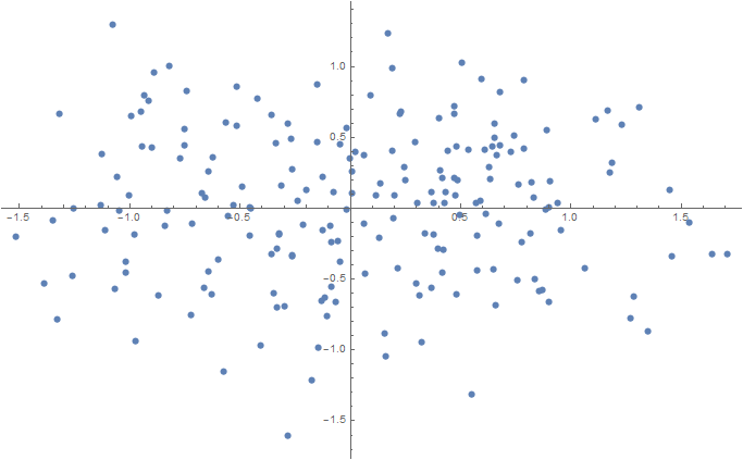
Num = 100; sigma = 0.1; data2D = Join[ f[{0.5, 0}, {sigma, sigma}, Num], f[{-0.5, 0}, {sigma, sigma}, Num] ]; ListPlot[data2D] Export[NotebookDirectory[] <> "data2D.csv", data2D, "CSV"]; 3D (projection onto two-dimensional space using t-SNE)
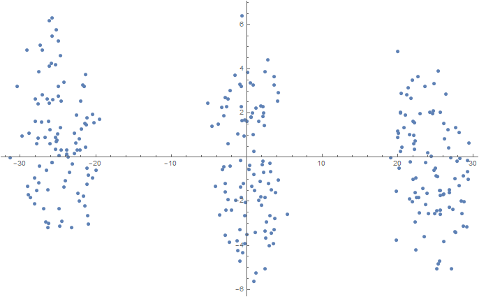
Num = 100; mu1 = 0.0; sigma1 = 0.1; mu2 = 2.0; sigma2 = 0.2; mu3 = 5.0; sigma3 = 0.3; data3D = Join[ f[{mu1, mu1, mu1}, {sigma1, sigma1, sigma1}, Num], f[{mu2, mu2, mu2}, {sigma2, sigma2, sigma2}, Num], f[{mu3, mu3, mu3}, {sigma3, sigma3, sigma3}, Num] ]; dimReducer = DimensionReduction[data3D, Method -> "TSNE"]; ListPlot[dimReducer[data3D]] Export[NotebookDirectory[] <> "data3D.csv", data3D, "CSV"]; 5D (projection onto two-dimensional space using t-SNE)

Num = 250; mu1 = -2.5; sigma1 = 0.9; mu2 = 0.0; sigma2 = 1.5; mu3 = 2.5; sigma3 = 0.9; data5D = Join[ f[{mu1, mu1, mu1, mu1, mu1}, {sigma1, sigma1, sigma1, sigma1, sigma1}, Num], f[{mu2, mu2, mu2, mu2, mu2}, {sigma2, sigma2, sigma2, sigma2, sigma2}, Num], f[{mu3, mu3, mu3, mu3, mu3}, {sigma3, sigma3, sigma3, sigma3, sigma3}, Num] ]; dimReducer = DimensionReduction[data5D, Method -> "TSNE"]; ListPlot[dimReducer[data5D]] Export[NotebookDirectory[] <> "data5D.csv", data5D, "CSV"]; And "run them" through both algorithms building a cluster. The results obtained are summarized in the table:
| 2D | 3D | 5D | |
|---|---|---|---|
| Clusterization Quality (via K-Means): | 90.30318857796479 | 96.48947132305597 | 1761.3743823022821 |
| Clusterization Quality (via Optimization): | 87.42370021528419 | 96.4552486768293 | 1760.993575500699 |
Clusterizer Results
2D
3D (projection onto two-dimensional space using t-SNE)
5D (projection onto two-dimensional space using t-SNE)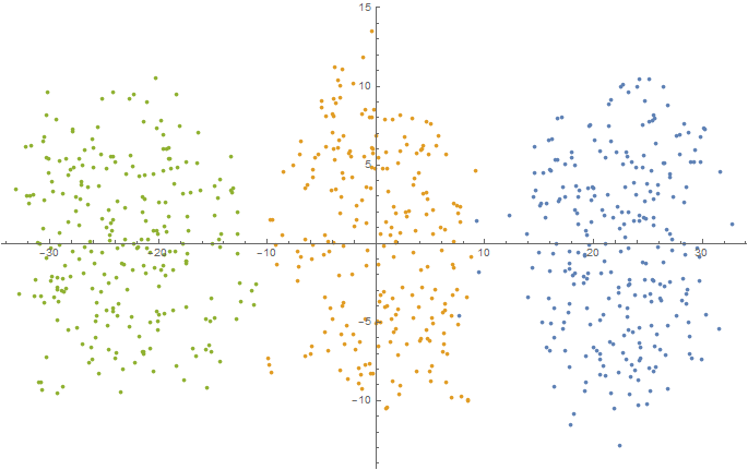
The table shows that even a simple optimization algorithm can successfully solve the problem of constructing a simple clusterizer. At the same time, the created clusterizer will be optimal (and to be honest, suboptimal, since the optimization method used does not guarantee finding the global optimum point) in terms of the quality metric used. Naturally, the optimization algorithm used for problems of a higher dimension is hardly suitable (here it is better to use more complex and efficient algorithms based on several heuristics of different levels). For a small synthetic task, Random Search did quite well.
Instead of an afterword
I would like to thank everyone who read the article, unsubscribed in the comments. In short, everyone who contributed to the creation of this work. Probably, it should be immediately noted that articles on this subject will appear as far as possible and my current workload. But I would like to say that this time I will try to bring the matter begun by me to the end.
References and literature
Source: https://habr.com/ru/post/328198/
All Articles