A simple model of the adaptive Kalman filter by means of Python

Problem

The eternal problem of any measurement is their low accuracy. There are two main ways to increase accuracy, the first is to increase the sensitivity to the measured value, however, this usually increases the sensitivity to non-informative parameters, which requires additional measures to compensate for them. The second method consists in statistical processing of multiple measurements, while the standard deviation is inversely proportional to the square root of the number of measurements.

Statistical methods for improving accuracy are diverse and numerous, but they are also divided into passive for static measurements and active for dynamic measurements when the measurable value changes over time. In this case, the measured value itself, as well as the interference, are random variables with varying dispersions.

The adaptability of methods to improve the accuracy of dynamic measurements should be understood as the use of prediction of the values of variances and errors for the next measurement cycle. Such prediction is carried out in each measurement cycle. For this purpose, apply Wiener filters operating in the frequency domain. Unlike the Wiener filter, the Kalman filter works in the time domain and not in the frequency domain. The Kalman filter was developed for multidimensional problems, the formulation of which is carried out in a matrix form. The matrix form is described in sufficient detail for implementation in Python in the article [1], [2]. The description of the work of the Kalman filter given in these articles is intended for specialists in the field of digital filtering. Therefore, it became necessary to consider the operation of the Kalman filter in a simpler scalar form.

Some theory

Consider the Kalman filter scheme for its discrete form.

Here G (t) block whose operation is described by linear relations. The output of the block produces a non-random signal y (t). This signal is summed with the noise w (t), which occurs inside the controlled object. As a result of this addition, we obtain a new signal x (t). This signal represents the sum of the non-random signal and noise and is a random signal. Further, the signal x (t) is transformed by the linear block H (t), summing up with the noise v (t), which is distributed differently than w (t) to the law. At the output of the linear block H (t), we get a random signal z (t), which is used to determine the non-random signal y (t). It should be noted that the linear functions of the blocks G (t) and H (t) may also depend on time.
')
We assume that random noise w (t) and v (t) are random processes with variances Q, R and zero mathematical expectations. The signal x (t) after a linear transformation in the G (t) block is distributed in time according to the normal law. Taking into account the above, the ratio for the measured signal will take the form:

z (t) = H (x (t)) + v (t)

$z (t) = H (x (t)) + v (t)$

Formulation of the problem

After the filter, you need to get the maximum possible approximation of y "to the non-random signal y (t).

With continuous dynamic measurement, each next state of the object, and, consequently, the value of the monitored quantity differs from the previous one exponentially with a constant time T in the current time interval

Below is a Python program that solves an equation for an unknown, non-noisy signal y (t). The measurement process is considered for the sum of two pseudo-random variables, each of which is formed as a function of the normal distribution of a uniform distribution.

The program for the demonstration of the discrete adaptive filter Kalman

#!/usr/bin/env python #coding=utf8 import matplotlib.pyplot as plt import numpy as np from numpy import exp,sqrt from scipy.stats import norm Q=0.8;R=0.2;y=0;x=0#  ( )    . P=Q*R/(Q+R)#    . T=5.0# . n=[];X=[];Y=[];Z=[]#  . for i in np.arange(0,100,0.2): n.append(i)# . x=1-exp(-1/T)+x*exp(-1/T)#   x. y=1-exp(-1/T)+y*exp(-1/T)#    y. Y.append(y)#   y. X.append(x)#    x. norm1 = norm(y, sqrt(Q))#    #  – y. norm2 = norm(0, sqrt(R))# ))#    #  – 0. ravn1=np.random.uniform(0,2*sqrt(Q))#  #    Q. ravn2=np.random.uniform(0,2*sqrt(R))#   #    R. z=norm1.pdf( ravn1)+norm2.pdf( ravn2)#  z. Z.append(z)#    z. P=P-(P**2)/(P+Q+R) #     x. x=(P*z+x*R)/(P+R)#   x. P=(P*R)/(P+R)#     x. plt.plot(n, Y, color='g',linewidth=4, label='Y') plt.plot(n, X, color='r',linewidth=4, label='X') plt.plot(n, Z, color='b', linewidth=1, label='Z') plt.legend(loc='best') plt.grid(True) plt.show()

What is the difference between the proposed algorithm and the known

I have improved the algorithm of the Kalman filter, given in the guidelines [3] for Mathcad:

As a result of a premature change of state for the compared variable x (t), the error in the area of abrupt changes increased:

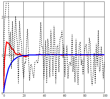
Whereas in my algorithm, an initial predictive estimate of the influence of noise is used. This made it possible to reduce the measurement error v (t).

In the given algorithm, the specified model model exponential functions are used, so for clarity, we present them separately on the general schedule of the Kalman filter.

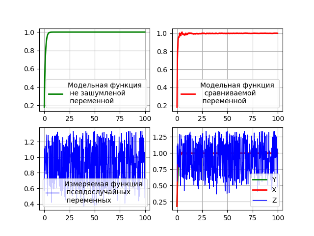
Program code for graphic analysis of the filter

 #!/usr/bin/env python #coding=utf8 import matplotlib.pyplot as plt import numpy as np from numpy import exp,sqrt from scipy.stats import norm Q=0.8;R=0.2;y=0;x=0#  ( )    . P=Q*R/(Q+R)#    . T=5.0# . n=[];X=[];Y=[];Z=[]#  . for i in np.arange(0,100,0.2): n.append(i)# . x=1-exp(-1/T)+x*exp(-1/T)#   x. y=1-exp(-1/T)+y*exp(-1/T)#    y. Y.append(y)#   y. X.append(x)#    x. norm1 = norm(y, sqrt(Q))#    #  – y. norm2 = norm(0, sqrt(R))# ))#    #  – 0. ravn1=np.random.uniform(0,2*sqrt(Q))#  #    Q. ravn2=np.random.uniform(0,2*sqrt(R))#   #    R. z=norm1.pdf( ravn1)+norm2.pdf( ravn2)#  z. Z.append(z)#    z. P=P-(P**2)/(P+Q+R) #     x. x=(P*z+x*R)/(P+R)#   x. P=(P*R)/(P+R)#     x. plt.subplot(221) plt.plot(n, Y, color='g',linewidth=2, label='  \n   \n ') plt.legend(loc='best') plt.grid(True) plt.subplot(222) plt.plot(n, X, color='r',linewidth=2, label='  \n  \n ') plt.legend(loc='best') plt.grid(True) plt.subplot(223) plt.plot(n, Z, color='b', linewidth=1, label='  \n  ') plt.legend(loc='best') plt.grid(True) plt.subplot(224) plt.plot(n, Y, color='g',linewidth=2, label='Y') plt.plot(n, X, color='r',linewidth=2, label='X') plt.plot(n, Z, color='b', linewidth=1, label='Z') plt.legend(loc='best') plt.grid(True) plt.show()

The result of the program

findings

The article describes a model of a simple scalar implementation of the Kalman filter by means of a conditionally free general-purpose programming language Python, which expands the scope of its application for learning purposes.

Links

Source: https://habr.com/ru/post/328146/

All Articles