Quake 2 source code overview
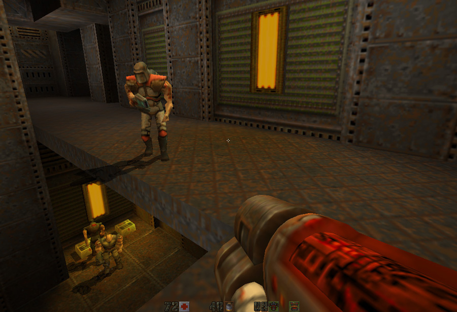
I spent about a month of free time reading the Quake II source code. It was an amazing and instructive experience, because a big change was made to idTech3: Quake 1, Quake World and QuakeGL are combined into one beautiful code architecture. Of particular interest was the way modularity was achieved, despite the fact that the C programming language does not provide polymorphism.
Quake II is in many ways a brilliant example of software, because it was the most popular (by the number of licenses) three-dimensional engine of all time. Based on it, more than 30 games were created. In addition, he marked the transition of the gaming industry from software / 8-bit color system to hardware / 24-bit. This transition occurred around 1997.
')
Therefore, I highly recommend everyone who loves programming to learn this engine. As usual, I kept an infinite number of notes, then cleaned them up and published them as an article to save you a few hours.
The process of “erasure” I was very fascinated: the article now has more than 40 megabytes of video, screenshots and illustrations. Now I don’t know if my works were worth it, and whether it’s necessary to publish in the future unprocessed notes in ASCII, express your opinion.
First meeting and compilation
The source code is freely available on the id Software ftp site . The project can be opened in Visual Studio Express 2008, which can also be freely downloaded from the Microsoft website.
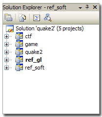
The first problem is that the working environment in Visual Studio 6 creates not one, but five projects. This is because Quake2 was developed modular (I will talk more about this later). Here is what comes out of the projects:
| Projects | Assembly |
| ctf | gamex86.dll |
| game | gamex86.dll |
| quake2 | quake.exe |
| ref_soft | ref_soft.dll |
| ref_gl | ref_gl.dll |
Note 2: first, the build fails due to the lack of a DirectX header:
fatal error C1083: Cannot open include file: 'dsound.h': No such file or directory I installed the Direct3D SDK and Microsoft SDK (for MFC), and everything compiled normally.
Software erosion: it looks like what happened to the Quake code base begins to happen with Quake 2: it’s impossible to open the work environment in Visual Studio 2010. You must use VS 2008.
Note: if an error occurs after compilation
"Couldn't fall back to software refresh!" ,This means that the renderer DLL could not be loaded correctly. But it is easy to fix:
Quake2 core loads two of its DLLs using win32 API: LoadLibrary. If the DLL is not the one that is expected or it is impossible to resolve the DLL dependencies, then the failure occurs without displaying an error message. Therefore:
- Connect all five projects with one library - right-click on each project -> properties -> C / C ++: make sure that “runtime library” = Multi-threaded Debug DLL (with “Debug” configuration, otherwise use release).
If you use the quake2 version released by id Software, this will eliminate the error.
- If you are using my version: I added the ability to save screenshots to PNG in the engine, so you need to also compile libpng and libz (they are in a subdirectory). Make sure the Debug DLL configuration is selected. When building, do not forget to place the libpng and zlib DLLs in the same folder as quake2.exe.
Quake2 architecture
When I read the Quake 1 code, I divided the article (its translation is here ) into three parts: “Network”, “Prediction” and “Visualization”. Such an approach would also be appropriate for Quake 2, because the engine is not very different in its core, but it is easier to notice the improvements if you divide the article into three main types of projects:
| Type of project | Project Information |
| Main engine (.exe) | The kernel that calls the modules and exchanges information between the client and the server. In a production environment, this is a quake2 project. |
| Renderer Module (.dll) | Responsible for visualization. The working environment contains the software renderer ( ref_soft ) and the OpenGL renderer ( ref_gl ). |
| Game Module (.dll) | Responsible for the gameplay (game content, weapons, monster behavior ...). The production environment contains a single-user module ( game ) and a module Capture The Flag ( ctf ). |
win32/sys_win.c . The WinMain method performs the following tasks: game_export_t *ge; // dll refexport_t re; // dll WinMain() // quake2.exe { Qcommon_Init (argc, argv); while(1) { Qcommon_Frame { SV_Frame() // { // if (!svs.initialized) return; // game.dll ge->RunFrame(); } CL_Frame() // { // if (dedicated->value) return; // renderer.dll re.BeginFrame(); //[...] re.EndFrame(); } } } } A completely disassembled cycle can be found in my notes.
You may ask: "why do we need such changes in architecture?". To answer this question, let's look at all versions of Quake from 1996 to 1997:
- Quake
- WinQuake.
- GLQuake.
- Vquake (a few words from one of the developers Stefan Podell (Stefan Podell) about the difficulties of the V2200 in Z-buffering ( mirror )).
- Quake World Server.
- Quake World Client.
Many executable files were created, and each time it was required to fork or configure the code through the
#ifdef preprocessor. It was a complete chaos, and to get rid of it, it was necessary:- Unify client / server.
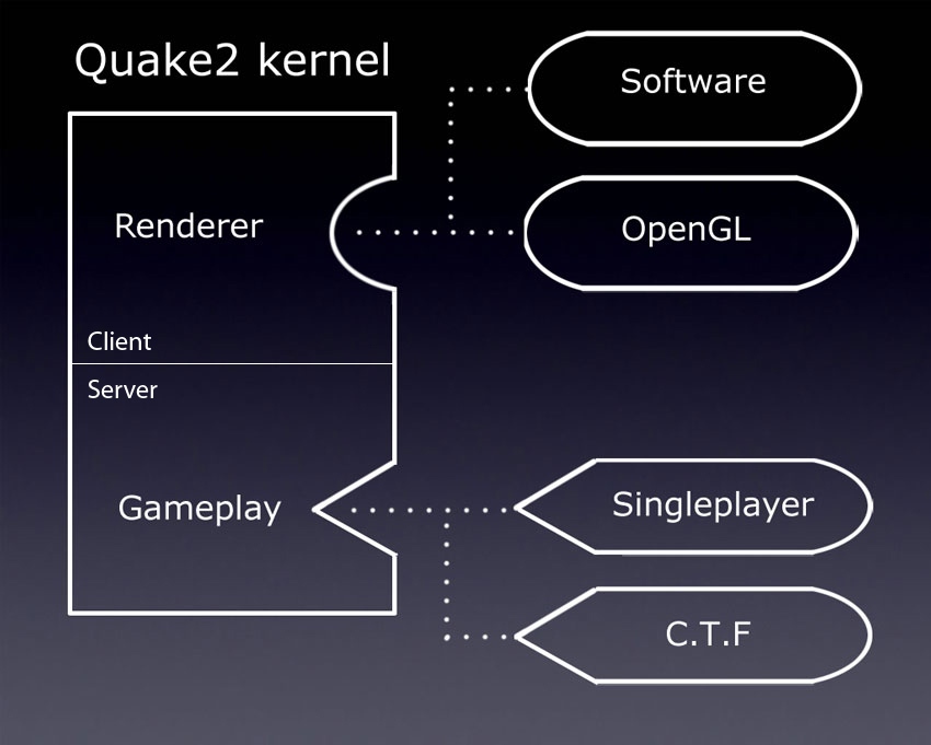
- Build a kernel capable of loading interchangeable modules.
A new approach can be illustrated in this way:
Two major improvements:
- Client-server unification: there was no longer one exe for the client and another for the server, the main executable file could work as a server, client, or both. Even in single-user mode, the client and server were still running in the same executable file (although in this case the data was exchanged via a local buffer, and not via TCP IP / IPX).
- Modularity: thanks to the dynamic connection, part of the code has become interchangeable. The renderer and game code became modules that could be switched without changing the core of Quake2. Thus, polymorphism was achieved using two structures containing function pointers.
These two changes made the code base extremely elegant and more readable than Quake 1, which suffered from code entropy.
From the point of view of implementation, DLL projects should disclose only one method
GetRefAPI for renderers and GetGameAPI for a game (look at the GetGameAPI file in the “Resource Files” folder):reg_gl/Resource Files/reg_soft.def EXPORTS GetGameAPI When the kernel needs to load a module, it loads the DLL into the process space, gets the
GetRefAPI address from GetProcAddress , gets the necessary function pointers and that's it.An interesting fact: in the local game, the connection between the client and the server is not performed through sockets. Instead, the commands are dropped into the “loopback” buffer using the
NET_SendLoopPacket in the client side of the code. The server reconstructs the command from the same buffer using the NET_GetLoopPacket .Random fact: if you have ever seen this photo, you probably wondered what John Carmack used for the giant display around 1996:

It was a 28-inch InterView 28hd96 monitor manufactured by Intergraph. This brute provided a resolution of up to 1920x1080, which is quite impressive for 1995 (you can read more here ( mirror )).
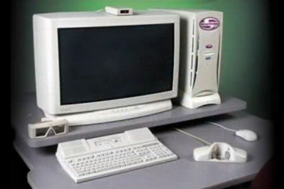
Nostalgic Youtube Video: Intergraph Computer Systems Workstations .
Addition: it looks like this article inspired someone on geek.com because they wrote the article “John Carmack created Quake in 1995 on a 28-inch 16: 9 1080p monitor” ( mirror ).
Addition: it seems that John Carmack still used this monitor when developing Doom 3.
Visualization
The modules of the software renderer (
ref_soft ) and the hardware accelerated renderer ( ref_gl ) were so large that I wrote separate sections about them.Again, it is noteworthy that the kernel did not even know which renderer is connected: it simply caused the function pointer in the structure. That is, the visualization pipeline was completely abstracted: and who needs this C ++?
Interesting fact: id Software still uses the coordinate system from the 1992 Wolfenstein 3D game (at least that's how it was in Doom3). This is important to know when reading the source code of the renderer:
In system id:
- X axis = left / right
- Y axis = front / rear
- Z axis = up / down
In the OpenGL coordinate system:
- X axis = left / right
- Y axis = up / down
- Z axis = front / rear
Therefore, the OpenGL renderer uses the
GL_MODELVIEW matrix to “fix” the coordinate system in each frame using the R_SetupGL method ( glLoadIdentity + glRotatef ).Dynamic connection
Much can be said about kernel / module interactions: I have written a separate section on dynamic connectivity.
Modding: gamex86.dll
Reading this part of the project was not so interesting, but the rejection of Quake-C for the compiled module led to two good and one very bad consequences.
The bad:
- Portability has been sacrificed, the game module must be recompiled for different platforms with specific linker parameters.
Good:
- Speed: The Quake-C language of the Quake1 game was interpreted code, but the Quake2
gamex86.dlldynamic librarygamex86.dllis native. - Freedom: modders gained access to EVERYTHING, not just what was available through Quake-C.
An interesting fact: ironically, id Software has moved Quake3 back to using a virtual machine (QVM) for gaming, artificial intelligence and modding.
My quake2
During the hacking process, I changed the Quake2 source code a bit. I highly recommend adding a DOS console to see the
printf output in the process, rather than pause the game to learn the Quake console:Adding a DOS-style console to a Win32 window is quite simple:
// sys_win.c int WINAPI WinMain (HINSTANCE hInstance, HINSTANCE hPrevInstance, LPSTR lpCmdLine, int nCmdShow) { AllocConsole(); freopen("conin$","r",stdin); freopen("conout$","w",stdout); freopen("conout$","w",stderr); consoleHandle = GetConsoleWindow(); MoveWindow(consoleHandle,1,1,680,480,1); printf("[sys_win.c] Console initialized.\n"); ... } Since I was running Windows on a Mac using Parallels, it was difficult to press "printscreen" while playing the game. To create screenshots, I set the "*" key from the digital block:
// keys.c if (key == '*') { if (down) // ! Cmd_ExecuteString("screenshot"); } And finally, I added a lot of comments and diagrams. Here is the "my" complete source code:
archive
Memory management
Doom and Quake1 had its own memory manager called “Zone Memory Allocation”: at startup,
malloc executed and the memory block was controlled using a list of pointers. The Memory Zone could be marked for quick cleaning of the desired category of memory. Zone Memory Allocator ( common.c: Z_Malloc, Z_Free, Z_TagMalloc , Z_FreeTags ) remained in Quake2, but it is rather useless:- Markings are not used and memory allocation / release is performed on top of
mallocandfree(I have no idea why id Software decided to entrust this work to C Standard Library). - Overflow detector (using the constant
Z_MAGIC) is also never used.
It is still very useful to measure memory consumption due to the
size attribute in the header inserted before allocating each block of memory: #define Z_MAGIC 0x1d1d typedef struct zhead_s { struct zhead_s *prev, *next; short magic; short tag; // int size; } zhead_t; The surface caching system has its own memory manager. The amount of distributed memory depends on the resolution and is determined by a strange formula, which however, very effectively protects against garbage:
malloc : ============================== size = SURFCACHE_SIZE_AT_320X240; //1024*768 pix = vid.width*vid.height; if (pix > 64000) size += (pix-64000)*3; 
“Hunk allocator” is used to load resources (images, sounds and textures). It is pretty good, trying to use
virtualAlloc and correlate data with the size of the page (8 KB, despite the fact that 4 KB was used in Win98! What kind of things ?!).And finally, there are also a lot of FIFO stacks (among other things, for storing intervals) , and despite the obviously limited possibilities, they work very well.
Memory management: ordering trick
Because Quake2 manages many of the usual pointers, a good trick is used to place the pointer in 32 bits (or placement in 8 KB to minimize PAGE_FAULT ... despite the fact that Windows 98 used 4 KB pages).
The layout of the pages (8 KB):
int roundUpToPageSize(int size) { size = (size + 8191) & ~8191; return size; } Memory Location (4 B):
memLoc = (memLoc + 3) & ~3; // 4- . Console subsystem
The Quake2 core contains a powerful console system that actively uses pointer lists and linear search.
It has three types of objects:
- Commands: give a function pointer for the given string value.
- Cvar: store a string value for the specified string name.
- Nickname: provides a replacement for the given string value.
In terms of code, each type of object has a list of pointers:
cmd_function_t *cmd_functions // , : void (*)() . cvar_t *cvar_vars // , . cmdalias_t *cmd_alias // , . When each line is entered into the console, it is scanned, supplemented (using aliases and corresponding cvar), and then divided into tokens stored in two global variables:
cmd_argc and cmd_argv : static int cmd_argc; static char *cmd_argv[MAX_STRING_TOKENS]; Example:
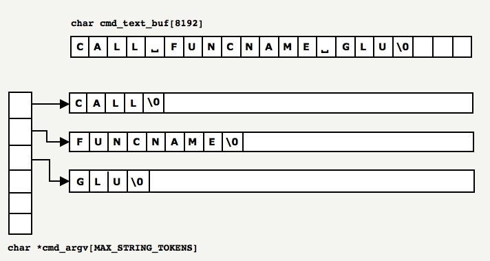
Each token identified in the buffer is copied
memcpy to the location indicated by malloc cmd_argv . The process is rather inefficient and shows that little attention was paid to this subsystem. And this, by the way, is fully justified: it is rarely used and has little effect on the game, so optimization was not worth the effort. The best approach would be to patch the source line in place and write the pointer value for each token:
Since the tokens are in the array of arguments,
cmd_argv[0] checked in a very slow and linear way to match all the functions declared in the list of function pointers. If a match is found, the function pointer is called.If no match is found, the list of alias pointers is linearly checked to determine if the token is a function call. If the alias replaces a function call, then it is called.
And finally, if none of the above work, then Quake2 processes the token as a variable declaration (or as its update, if the variable is already in the list of pointers).
There are many linear searches in the list of pointers: the ideal solution would be to use a hash table. It would allow O (n) complexity instead of O (n²).
An interesting fact about parsing 1 : the ASCII table is cleverly organized: when parsing a string to create tokens, you can skip delimiters and space characters simply by checking if the character i is smaller than the character '' (space).
char* returnNextToken(char* string) { while (string && *string < ' ') string++; return string; } An interesting fact about parsing 2 : the ASCII table was organized very cleverly: you could convert the character c to an integer as follows:
int value = c - '0';
int charToInt(char v) { return v - '0' ; } Caching cvar values:
Since the search for cvar in memory (
Cvar_Get ) in this system has O (n²) complexity (linear search + strcmp for each record), renderers cache the cvar in memory: // cvar_t *crosshair; // , // Cvar . crosshair = Cvar_Get ("crosshair", "0", CVAR_ARCHIVE); // // , . void SCR_DrawCrosshair (void) { if (!crosshair->value) // return; } Access to this value can then be obtained for O (1).
Protection from villains
To protect against cheating, several mechanisms were inserted:
- Even though UDP has its own CRC, Quake CRC (
COM_BlockSequenceCRCByte) is added to each packet to protect against modification. - Before the start of the dematch, levels are hashed using MD4. This hash is sent to the server to make sure that the client does not use modified cards (
Com_BlockChecksumM). - There is even a system that checks the number of teams per second from each player (
SV_ClientThink), but I do not know exactly how effective it was.
Internal assembler
As in every version of Quake, some of the useful functions were optimized using assembly language (however, there are still no traces of the famous “quick back square root” that was present in Quake3).
The fast absolute value of a 32-bit floating point number (most compilers today do this automatically):
float Q_fabs (float f) { int tmp = * ( int * ) &f; tmp &= 0x7FFFFFFF; return * ( float * ) &tmp; } Fast Float to Integer conversion
__declspec( naked ) long Q_ftol( float f ) { static int tmp; __asm fld dword ptr [esp+4] __asm fistp tmp __asm mov eax, tmp __asm ret } Code statistics
Analysis of the code in Cloc showed that there are a total of 138,240 lines in the code. As usual, this number does NOT give an idea of the effort invested, because much has been abandoned in the iterative cycle of engine versions, but, as it seems to me, this is a good indicator of the total engine complexity.
$ cloc quake2-3.21/ 338 text files. 319 unique files. 34 files ignored. http://cloc.sourceforge.net v 1.53 T=3.0 s (96.0 files/s, 64515.7 lines/s) ------------------------------------------------------------------------------- Language files blank comment code ------------------------------------------------------------------------------- C 181 24072 19652 107757 C/C++ Header 72 2493 2521 14825 Assembly 22 2235 2170 8331 Objective C 6 1029 606 4290 make 2 436 67 1739 HTML 1 3 0 1240 Bourne Shell 2 17 6 54 Teamcenter def 2 0 0 4 ------------------------------------------------------------------------------- SUM: 288 30285 25022 138240 ------------------------------------------------------------------------------- Note: the entire assembly code is designed for a manually created software renderer.
Tools recommended for working with Quake2 hacking
- Visual Studio Express 2008.
- Free Quake2 demo from website id.
- Pak explorer written by me.
- Wally : WAL image format viewer.
- The famous research tool pak ( PakExpl )
- An article about the BSP format ( mirror ) from the FlipCode website.
- Profilers C: VTune (intel), CodeAnalysis (AMD), Visual Studio Team Profiler (the best, in my opinion).
- Large 24/30 inch screen.
- Keyboard IBM Model M.
Quake2 consists of one core and two modules loaded during execution: Game and Renderer. It is very interesting that thanks to polymorphism, anything can be connected to the kernel.
Before continuing to read, I recommend to make sure that you understand the principle of the virtual memory well with the help of this wonderful article ( mirror ).
Polymorphism in C with dynamic connectivity
Dynamic connectivity offers many benefits:
- Renderer:
- Pure Quake2 kernel code, reduced code entropy, no crazy
#ifdefeverywhere. - The release of the game with several renderers (software, openGL).
- Renderer can be changed when playing the game.
- Ability to create a new renderer for equipment created after the release of the game (Glide, Verity).
- Pure Quake2 kernel code, reduced code entropy, no crazy
- Modding games:
- More options for authors of mods, the game can be completely changed through game.dll.
- Full game speed in mods, no need to rely on QuakeC and Quake Virtual Machine.
- No need to learn QuakeC, DLLs were written in C.
But Quake2 was written in C, which is not an object-oriented programming language, so the question was: "How to implement polymorphism in a language that is not OO?"
The technique of simulating OO is similar to the method used in Java and C ++: the use of structures containing function pointers.
Therefore, four structures were used to exchange function pointers:
refimport_t and refexport_t acted as a container for exchanging function pointers when loading the renderer module. game_import_t and game_export_t used when loading the game module.A small illustration is better than a long speech.
Step 1: Initially:
quake2.execontains theref_OpenGL_tstructure with function pointers toNULL(gray).- The DLL module (
ref_opengl.dll) also contains akernel_fct_tstructure with function pointers toNULL(gray).
The task of the process is to transfer the addresses of the functions so that each part can call the others.

Step 2: The kernel that calls the function fills the structure containing the pointers to its own functions and sends these DLL values.

Step 3: The host DLL copies the kernel function pointers and returns a structure containing its own function addresses.

The process with real names is described in detail in the next two sections.
Renderer Library
The method that gets the renderer module is called
VID_LoadRefresh . It is called every frame so that Quake can switch between renderers (but due to the pre-processing renderer, you need to restart the level).This is what happens on the Quake2 core side:
refexport_t re; qboolean VID_LoadRefresh( char *name ) { refimport_t ri; GetRefAPI_t GetRefAPI; ri.Sys_Error = VID_Error; ri.FS_LoadFile = FS_LoadFile; ri.FS_FreeFile = FS_FreeFile; ri.FS_Gamedir = FS_Gamedir; ri.Cvar_Get = Cvar_Get; ri.Cvar_Set = Cvar_Set; ri.Vid_GetModeInfo = VID_GetModeInfo; ri.Vid_MenuInit = VID_MenuInit; ri.Vid_NewWindow = VID_NewWindow; GetRefAPI = (void *) GetProcAddress( reflib_library, "GetRefAPI" ); re = GetRefAPI( ri ); ... } In the above code, the Quake2 kernel retrieves a pointer to the function of the method
GetRefAPIfrom the renderer DLL using GetProcAddress(built-in win32 method).Here is what happens in the
GetRefAPIrenderer DLL: refexport_t GetRefAPI (refimport_t rimp ) { refexport_t re; ri = rimp; re.api_version = API_VERSION; re.BeginRegistration = R_BeginRegistration; re.RegisterModel = R_RegisterModel; re.RegisterSkin = R_RegisterSkin; re.EndRegistration = R_EndRegistration; re.RenderFrame = R_RenderFrame; re.DrawPic = Draw_Pic; re.DrawChar = Draw_Char; re.Init = R_Init; re.Shutdown = R_Shutdown; re.BeginFrame = R_BeginFrame; re.EndFrame = GLimp_EndFrame; re.AppActivate = GLimp_AppActivate; return re; } At the end, a two-way exchange of data between the kernel and the DLL is established. It is polymorphic, because the renderer DLL returns its own function addresses inside the structure and the Quake2 kernel doesn’t see the difference, it always calls the same function pointer.
Game library
The exact same process is done with the kernel-side game library:
game_export_t *ge; void SV_InitGameProgs (void) { game_import_t import; import.linkentity = SV_LinkEdict; import.unlinkentity = SV_UnlinkEdict; import.BoxEdicts = SV_AreaEdicts; import.trace = SV_Trace; import.pointcontents = SV_PointContents; import.setmodel = PF_setmodel; import.inPVS = PF_inPVS; import.inPHS = PF_inPHS; import.Pmove = Pmove; // 30 ge = (game_export_t *)Sys_GetGameAPI (&import); ge->Init (); } void *Sys_GetGameAPI (void *parms) { void *(*GetGameAPI) (void *); //[...] GetGameAPI = (void *)GetProcAddress (game_library, "GetGameAPI"); if (!GetGameAPI) { Sys_UnloadGame (); return NULL; } return GetGameAPI (parms); } Here is what happens on the DLL side of the game:
game_import_t gi; game_export_t *GetGameAPI (game_import_t *import) { gi = *import; globals.apiversion = GAME_API_VERSION; globals.Init = InitGame; globals.Shutdown = ShutdownGame; globals.SpawnEntities = SpawnEntities; globals.WriteGame = WriteGame; globals.ReadGame = ReadGame; globals.WriteLevel = WriteLevel; globals.ReadLevel = ReadLevel; globals.ClientThink = ClientThink; globals.ClientConnect = ClientConnect; globals.ClientDisconnect = ClientDisconnect; globals.ClientBegin = ClientBegin; globals.RunFrame = G_RunFrame; globals.ServerCommand = ServerCommand; globals.edict_size = sizeof(edict_t); return &globals; } Using function pointers
After passing the method pointers, polymorphism is enabled. Here in the code, the kernel "jumps" to different modules: The
renderer "jumps" to
SCR_UpdateScreen: // quake.exe, , quake2.exe , . SCR_UpdateScreen() { // re - struct refexport_t, BeginFrame BeginFrame DLL. re.BeginFrame( separation[i] ); // DLL SCR_CalcVrect() SCR_TileClear() V_RenderView() SCR_DrawStats SCR_DrawNet SCR_CheckDrawCenterString SCR_DrawPause SCR_DrawConsole M_Draw SCR_DrawLoading re.EndFrame(); // quake.exe. } The game "jumps" to
SV_RunGameFrame: void SV_RunGameFrame (void) { sv.framenum++; sv.time = sv.framenum*100; // , if (!sv_paused->value || maxclients->value > 1) ge->RunFrame (); .... } } Software renderer
The Quake2 software renderer is the largest, most complex, and therefore the most interesting module for research.

There are no hidden mechanisms here, starting with the disk and ending with pixels.
All code is neatly written and optimized by hand. He is the last of its kind and marked the end of an era. Later, the industry completely switched exclusively to hardware accelerated rendering.
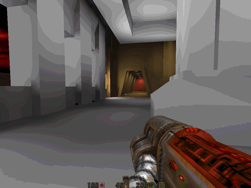
The fundamental difference between software rendering and rendering OpenGL - using the 256-color palette system instead of the usual 24-bit True Color RGB system today:

If we compare the hardware accelerated renderer and the software renderer, we notice two of the most obvious differences:
- Lack of color lighting
- No bilinear filtering
But with the exception of this, the engine managed to perform amazing work using the very clever use of the palette, which I will discuss later:
- Quick selection of color gradients (64 values).
- Fullscreen mixing of post-effect colors.
- Pixel translucency.
First, the Quake2 palette is loaded from the PAK archive file
pics/colormap.pcx:
Note: the black value is 0, the white is 15, the green is 208, the red is 240 (in the lower left corner), the transparent is 255.
First of all, the 256 colors are rearranged according to
pics/colormap.pcx:
This 256x320 scheme is used as a lookup table, and it is extremely clever, because it provides many interesting features:
- 64 : 256 «» . 63 , 255 . :
- [0,255] ( ).
- x*256, x [0,63] ( ).
64 256 . 256 . Awesome - The rest of the image is created from 16x16 squares, which allows you to use pixel blending based on a palette. It is clearly visible that all the squares are created from the original color, the final color and intermediate colors. This is how water translucency is realized in the game. For example, black and white are mixed in the upper left square.
Interesting fact: the Quake2 software renderer was originally based on MMX technology and should have been based on RGB, not on the palette, as John Carmack said after the release of Quake1 in this video (moment at 10 minute 17 second):
MMX is a SIMD technology that allows you to work with all three RGB channels at the cost of just one channel, thus providing mixing with acceptable CPU consumption. I assume that it was abandoned for the following reasons:
- Pentium MMX 1997 , .
- RGB (16 32 ) (8 ) , .
Having defined the main constraint (palette), you can go to the general architecture of the renderer. His philosophy used Pentium's strengths (floating-point calculations) to reduce the effect of weaknesses: bus speed, which influenced the recording of pixels in memory. Most of the rendering path is focused on achieving zero redrawing. In essence, the software rendering path is similar to the Quake 1 software rendering method. It used BSP and PVS (a set of potentially visible polygons) to bypass the map to get a set of polygons that need to be rendered. Each frame renders three different elements:
- Map: using the coherent line-by-line image construction algorithm based on BSP (more about it later).
- Entities: either as “sprites” (windows), or as “objects” (players, enemies) using a simple line-by-line image creation algorithm.
- Particles
Note: If you are not familiar with these “old” algorithms, I highly recommend reading chapters 3.6 and 15.6 of Computer graphics: principles and practice of James D. Foley. You can also find a lot of information in chapters 59-70 of Michael Abrash's Graphics programming black book .
Here is the high level pseudocode:
- Rendering maps
- Passing through a pre-processed BSP tree to determine the cluster in which we are.
- Query the PVS database about this particular cluster: getting and unpacking the PVS.
- PVS: , , .
- BSP. , - . , .
- :
- BSP, :
- : .
- (=+ ) .
- ( ).
- . . Z-.
- BSP, :
- , Z- .
- .
- .
- ( ).
Screen visualization: palette indexes are written to the voice-over buffer. Depending on the mode (fullscreen / windowed), DirectDraw or GDI is used. After the frame-by-frame buffer is completed, it is transferred to the video card's on-screen buffer (GDI =>
rw_dib.cDirectDraw =>rw_ddraw.c) using eitherBitBlt WinGDI.horBltFast ddraw.h.DirectDraw or GDI
Those problems that programmers had to meet in 1997 were simply depressing: John Carmack left a funny comment in the source code:
// DIB If Quake2 was working in full screen mode with DirectDraw, it had to draw the offscreen buffer from top to bottom: that was how it was displayed on the screen. But when it was executed in windowed mode with GDI, it was necessary to draw the voice-over buffer in the DIB buffer ... reflected vertically, because most of the drivers for video card manufacturers transferred the DIB image from RAM to the video memory in reflected mode (one wonders if I really in the acronym GDI stands for "Independent").
Therefore, the transition to the frame-by-frame buffer was supposed to become abstract. We needed a structure and values that were initialized differently to abstract from these differences. This is a primitive way to implement polymorphism in C.
typedef struct { pixel_t *buffer; // pixel_t *colormap; // : 256 * VID_GRADES pixel_t *alphamap; // : 256 * 256 int rowbytes; // , // DIB int width; int height; } viddef_t; viddef_t vid ; Depending on the method required to render the frame buffer, it was
vid.bufferinitialized as the first pixel:- First line for DirectDraw
- Last line for WinGDI / DBI
To go up or down,
vid.rowbytesinitialized as vid.widthor as -vid.width.

Now for the transition it does not matter how the drawing is performed: normal or with vertical reflection:
// byte* pixel = vid.buffer + vid.rowbytes * 0; // pixel = vid.buffer + vid.rowbytes * (vid.height-1); // i ( 0) pixel = vid.buffer + vid.rowbytes * i; // memset(vid.buffer,0,vid.height*vid.height) ; // <-- DirectDraw // ! This trick allows the rendering pipeline to not worry about how the transfer is performed at the lower level, and I think this is quite remarkable.
Preprocessing card
Before digging deeper into the code, you need to understand two important databases generated by preprocessing the map:
- Binary partitioning of space (BSP) / set of potentially visible polygons (PVS).
- Radiation-based lighting map texture.
Cutting BSP, generating PVS
I recommend to study deeper the binary partitioning of space:
- Wikipedia ( in Russian ).
- Article The Idea of BSP Trees by Michael Abrash.
- Article Compiling BSP Trees by Michael Abrash.
- An ASCII-style article, an old bible .
As in Quake1, Quake2 cards undergo serious preliminary processing: their volume is recursively cut as in the figure below:
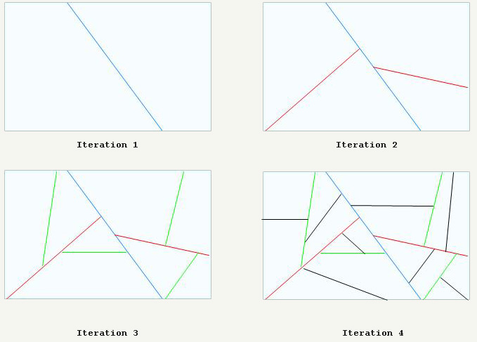
In the end, the card is completely cut into convex 3D spaces (called clusters). As in Doom with Quake1, they can be used to sort all polygons from front to back and from behind to the front.
A great addition is PVS, a set of bit vectors (one per cluster). Treat it as a database to which you can query and retrieve clusters that are potentially visible from any cluster. This database is huge (5 MB), but effectively compressed to several hundred kilobytes and fits well into RAM.
Note: compression is used for PVS compression, passing only 0x00 values, this process is explained below.
Radiation
As in Quake1, the effect of level lighting is calculated in advance and stored in textures called light maps. However, unlike Quake1, Quake2 uses radiation and color illumination in preliminary calculations. The lighting maps are then stored in the archive
PAKand used in the process of playing the game:A couple of words from one of the creators: Michael Abrash in Black Book of Programming (chapter “Quake: a post-mortem and a glimpse into the future”):
The most interesting graphics changes consisted in preliminary calculations, where John added support for the emitted light ...
Processing Quake 2 levels took up to an hour.
(However, it is worth noting that it included the creation of BSP, the calculation of PVS and the emitted light, which I will consider later.)
If you want to know about the radiated light, then read this stunningly well-illustrated article ( mirror ): this is just a masterpiece.
Here is the first level with a superimposed radiation texture: unfortunately, the stunning RGB colors needed to be resampled for a software renderer in grayscale (more on this later).
The low resolution of the irradiance map is striking here, but since it passes bilinear filtering (yes, even in the software renderer), the final result combined with the color texture is very good.
Interesting fact: lighting maps can be any size from 2x2 to 17x17 (despite the stated maximum size of 16 in the flipcode article ( mirror )) and do not have to be square.
Code architecture
Most software renderer code is in the method
R_RenderFrame. Here is a brief description, a more detailed analysis, read in my preliminary notes .R_SetupFrame: gets current viewpoint by BSP bypass (callMod_PointInLeaf), saves the viewpoint's clusterID tor_viewcluster.R_MarkLeaves: for the current review cluster (r_viewcluster) retrieves and unzips the PVS. Uses PVS to mark visible faces.R_PushDlights: uses BSP again to traverse faces from front to back. If the face is marked as visible, it checks if the light affects it.R_EdgeDrawing: level visualization.R_RenderWorld: BSP bypass front to back- Projecting all visible polygons into screen space: building a global edge table.
- ( ).
R_ScanEdges: , . :R_InsertNewEdges: , .(*pdrawfunc)(): , . . .D_DrawSurfaces: , .
R_DrawEntitiesOnList: , BModel (BModel — ). (, , )...R_DrawAlphaSurfaces:R_CalcPalette: calculation of post-effects, for example, mixing colors (when receiving damage, collecting items, etc.)
R_RenderFrame { R_SetupFrame // pdrawfunc , : GDI DirectDraw { Mod_PointInLeaf // , ( BSP-) r_viewcluster } R_MarkLeaves // (r_viewcluster) // PVS R_PushDlights // , , dlight_t* r_newrefdef.dlights. // R_EdgeDrawing // { R_BeginEdgeFrame // pdrawfunc, R_RenderWorld // // (surf_max - ) R_DrawBEntitiesOnList// , . R_ScanEdges // : // Z- ( ) { for (iv=r_refdef.vrect.y ; iv<bottom ; iv++) { R_InsertNewEdges // AET GET (*pdrawfunc)(); // D_DrawSurfaces // } // R_InsertNewEdges // AET GET (*pdrawfunc)(); // D_DrawSurfaces // } } R_DrawEntitiesOnList // , .... // Z- . R_DrawParticles // ! R_DrawAlphaSurfaces // <code>pics/colormap.pcx</code>. R_SetLightLevel // ( !) R_CalcPalette // ( ), } R_SetupFrame: BSP Management
Traversing the binary tree of space is performed throughout the code. This is a powerful mechanism with stable speed, allowing you to sort polygons from front to back or from behind. To understand it, you need to understand the structure
cplane_t: typedef struct cplane_s { vec3_t normal; float dist; } cplane_t; To calculate the distance or point from the section plane in a node, simply insert its coordinates into the equation of the plane:
int d = DotProduct (p,plane->normal) - plane->dist; Thanks to the sign
dwe find out whether we are in front of or behind the plane, and we can perform the sorting. This process has been used in engines starting with Doom and ending with Quake3.R_MarkLeaves: group unzipping of PVS
The way I understood the decompression of PVS in my analysis of the Quake 1 source code was completely wrong: it is not the distance between bits 1 that is encoded, but only the number of 0x00 bytes to be written. In PVS, only group compression 0x00 is performed: when reading a compressed stream:
- If a non-zero byte is read from compressed PVS, it is written to the unzipped version.
- If byte 0x00 is read from compressed PVS, then the next byte shows how many bytes to skip.
In the first case, nothing is compressed. Group compression is performed only in the second case:
byte *Mod_DecompressVis (byte *in, model_t *model) { static byte decompressed[MAX_MAP_LEAFS/8]; // = 1 , 65536 / 8 = 8 192 // PVS. int c; byte *out; int row; row = (model->vis->numclusters+7)>>3; out = decompressed; do { if (*in) // , . { *out++ = *in++; continue; } c = in[1]; // "", : (in[1]) in += 2; // PVS. while (c) { *out++ = 0; c--; } } while (out - decompressed < row); return decompressed; } You can skip up to 255 bytes (255 * 8 leaves), if necessary, after them you need to again add a zero with the number that you want to skip next 255 bytes. That is, the pass 511 bytes (511 * 8 leaves) takes 4 bytes: 0 - 255 - 0 - 255
Example:
// 80 , 10 : =1, =0 PVS 0000 0000 0000 0000 0000 0000 0000 0000 0011 1100 1011 1111 0000 0000 0000 0000 0000 0000 0000 0000 PVS 0x00 0x00 0x00 0x00 0x39 0xBF 0x00 0x00 0x00 0x00 // !! !! PVS 0000 0000 0000 1000 0011 1100 1011 1111 0000 0000 0000 1000 PVS 0x00 0x04 0x39 0xBF 0x00 0x04 After unpacking the PVS of the current cluster, each individual face belonging to the cluster that is considered visible in PVS is also marked as visible:
Q: How can I check the visibility of a cluster with a given identifier
iusing unzipped PVS?: bit AND between byte i / 8 PVS and 1 << (i% 8)
char isVisible(byte* pvs, int i) { // i>>3 = i/8 // i&7 = i%8 return pvs[i>>3] & (1<<(i&7)) } Just like in Quake1, there is a good trick used to mark the polygon as visible: instead of using flags and resetting each one at the beginning of each frame, it applies
int. At the beginning of each frame, the frame counter is r_visframecountincremented by one in R_MarkLeaves. After unpacking the PVS, all zones are marked as visible by assigning a visframecurrent value to the field r_visframecount.Later in the code, the visibility of the node / cluster is always checked in the following way:
if (node->visframe == r_visframecount) { // } R_PushDlights: dynamic lighting
For each identifier lightID of the active dynamic light source, a recursive BSP traversal is performed starting from the position of the light source. The distance between the source and the cluster is calculated, and if the illumination intensity is greater than the distance from the cluster, then all surfaces in the cluster are marked as affected by this source identifier.
Note: surfaces are marked with two fields:
dlightframe- this is the flagintused in the same way as in the case of marking the visibility of clusters (instead of resetting all the flags in each frame, the global variable increasesr_dlightframecount. For the light to affect, itr_dlightframecountmust be equal tosurf.dlightframe.dlightbitsIs a bit vectorintused to store indices of various arrays of light sources acting on a given face.
R_EdgeDrawing: level visualization
R_EdgeDrawing- This is a monster software renderer, the most difficult to understand. To deal with it, you need to look at the basic data structure:The stack
surf_t(acting as a proxy m_surface_t) is placed on the CPU stack.
// surf_t *surfaces ; // surf_t *surface_p ; // surf_t *surf_max ; // // bsp- " ", // , // surfaces[1] , Note: surfaces - Note: surfaces - This stack is filled when traversing a BSP from front to back. Each visible polygon is inserted into the stack as a proxy surface. Later, when traversing the table of active edges to generate a screen row, it allows you to very quickly see which polygon is in front of everyone else by comparing the address in memory (the lower the stack, the closer to the viewpoint). This is how “connectivity” is realized for the algorithm for converting line-by-line image construction.
Note: each stack item also has a list of pointers (called a chain of textures) pointing to items in the interval buffer stack (discussed below). Intervals are stored in a buffer and drawn from a chain of textures for deeply grouping intervals and maximizing the CPU pre-caching buffer.
The stack is initialized at the very beginning
R_EdgeDrawing: void R_EdgeDrawing (void) { // : 64 surf_t lsurfs[NUMSTACKSURFACES +((CACHE_SIZE - 1) / sizeof(surf_t)) + 1]; surfaces = (surf_t *) (((long)&lsurfs[0] + CACHE_SIZE - 1) & ~(CACHE_SIZE - 1)); surf_max = &surfaces[r_cnumsurfs]; // 0 ; , 0 // , , surfaces--; R_SurfacePatch (); R_BeginEdgeFrame (); // surface_p = &surfaces[2]; // - 1, // 0 - R_RenderWorld { R_RenderFace } R_DrawBEntitiesOnList R_ScanEdges // Z- ( ) { for (iv=r_refdef.vrect.y ; iv<bottom ; iv++) { R_InsertNewEdges // AET GET (*pdrawfunc)(); // D_DrawSurfaces // } // R_InsertNewEdges // AET GET (*pdrawfunc)(); // D_DrawSurfaces // } } Here are the details:
R_BeginEdgeFrame: clears the global edge table from the last frame.R_RenderWorld: BSP bypass (note that it does NOT render anything on the screen):- Each surface, which is considered visible, is added to the stack with a proxy
surf_t. - Projecting the vertices of all polygons to the screen space and filling the global edge table.
- Also generating a 1 / Z value for all vertices so that the Z-buffer can be generated at intervals.
- Each surface, which is considered visible, is added to the stack with a proxy
R_DrawBEntitiesOnList: I have no idea what this fragment does.R_ScanEdges: combining all the information received at the moment to render the level:- Initialization of the active edge table.
- Initialization of the interval buffer (also a stack):

// espan_t *span_p; // espan_t *max_span_p; // . span_p , // : (basespans) void R_ScanEdges (void) { int iv, bottom; byte basespans[MAXSPANS*sizeof(espan_t)+CACHE_SIZE]; ... } - Launching the line-by-line image algorithm from top to bottom on the screen.
- For each line:
- Updating the active edge table from the global edge table.
- Run the table of active edges for the whole row:
- The definition of the visible polygon using the address in the stack surfaces.
- Transfer interval to interval buffer.
- If the interval buffer is full: drawing all intervals and resetting the interval stack.
- Check remaining intervals in the buffer. If there is something left in it: drawing all the intervals and resetting the stack of intervals.
R_EdgeDrawing video
In the video below, the engine works with a resolution of 1024x768. It is also slowed down using a special cvar
sw_drawflat 1, which allowed rendering polygons without textures, but in different colors:In this video you can see a lot of interesting things:
- The screen is generated from top to bottom; this is a typical algorithm for line-by-line imaging.
- , . Pentium: textureId , « ». . , .
- , .
- , : , .
- 40% , 10%. , , .
- OMG, .
:
Unfortunately, beautiful 24-bit RGB lighting maps need to be resampled to 6-bit grayscale (by selecting the brightest channel from R, G, and B) to meet the palette restrictions:
What is stored in the archive
PAK(24 bits):After downloading from disk and resampling to 6-bit:
And then all together: the texture of the face gives the color in the range [0,255]. This value indexes the color in the palette from
pics/colormap.pcx:
Lighting maps are filtered: as a result, we get a value in the range [0.63].

Now using the top of the
pics/colormap.pcxslider can select the desired position of the palette. To get the final result, it uses the input value of the texture as the X coordinate and the illumination * 63 as the Y coordinate:
And voila:

Personally, I think it's amazing: imitation of 64 gradients of 256 colors ... only 256 colors!
Surface subsystem
From the previous screenshots it is obvious that the generation of surfaces is the most demanding of the CPU part of Quake2 (this is confirmed by the results of the profiler below). Acceptable with respect to speed and memory consumption, the generation of surfaces provides two mechanisms:
- MIP texturing (mipmapping)
- Caching
Surface subsystem: MIP texturing
When a polygon is projected into the screen space, 1 / Z of its distance is generated. The nearest vertex is used to determine which level of MIP textures to use. Here is an example of the lighting map and how it is filtered according to the level of the MIP textures:


Here is a mini-project I worked on to test the quality of Quilke2 bilinear filtering on random images: an archive .
Below are the results of a test performed for a 13x15 texel lighting map:

Level 3 of MIP textures: the block is 2x2 texels.

Level 2 MIP-textures: the block is 4x4 texel.

Level 1 MIP-textures: the block is 8x8 texels.

Level 0 MIP textures: the block is 16x16 texels.
The key to understanding filtering is that everything is based on the size of polygons in the space of the world (width and height are called
extent):- The Quake2 preprocessor ensures that the size of the polygon (X or Y) is less than or equal to 256, and is also a multiple of 16.
- From the size of the polygon in the space of the world, we can derive:
- Size of lightmap (in texels): LmpDim = PolyDim / 16 + 1
- Surface size (in blocks): SurDim = LmpDim -1 = PolyDim / 16
In the figure below, the dimensions of the polygon (3.4), the lighting maps are (4.5) texels, and the degenerate surface always has the size (3.4) of the block. Levels of MIP-textures determine the size of the block in texels, and hence the total size of the surface in texels.

All this is done in
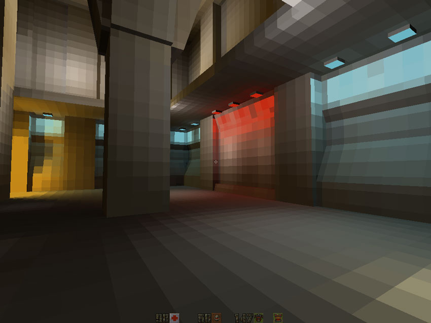
R_DrawSurface. The level of MIP-textures is selected using an array of function pointers ( surfmiptable), which selects the desired rasterization function: static void (*surfmiptable[4])(void) = { R_DrawSurfaceBlock8_mip0, R_DrawSurfaceBlock8_mip1, R_DrawSurfaceBlock8_mip2, R_DrawSurfaceBlock8_mip3 }; R_DrawSurface { pblockdrawer = surfmiptable[r_drawsurf.surfmip]; for (u=0 ; u<r_numhblocks; u++) (*pblockdrawer)(); } In the modified engine below you can see three levels of MIP-textures: 0 - gray, 1 - yellow and 2 - red:
Filtering is performed by the block when generating a block [i] [j] surface, the filter uses the values of the light map: lightmap [i] [ j], lightmap [i + 1] [j], lightmap [i] [j + 1] and lightmap [i + 1] [j + 1]: in essence, using four texels directly in the coordinates and three below and to the right . Notice that this is not done by weight interpolation, but rather linear interpolation, first vertically and then horizontally on the generated values. In short, it works exactly the same as in the Wikipedia article on bilinear filtering.
And now all together:

Original lighting map, 13x15 texels.

Filtering, level 0 of MIP-textures (16x16 blocks) = 192x224 texel.
Result:

Surface Subsystem: Caching
Even despite the fact that the engine is actively used to manage memory
mallocand freeit still uses its own memory manager for caching surfaces. The memory block is initialized immediately after the rendering resolution is known: size = SURFCACHE_SIZE_AT_320X240; pix = vid.width*vid.height; if (pix > 64000) size += (pix-64000)*3; size = (size + 8191) & ~8191; sc_base = (surfcache_t *)malloc(size); sc_rover = sc_base; Rover
sc_roverat the very beginning is located in the block to keep track of what was occupied. When the rover reaches the end of memory, it collapses, in effect, replacing old surfaces. The amount of reserved memory can be seen on the graph:
Here is how a new fragment of memory is allocated from the block:
memLoc = (int)&((surfcache_t *)0)->data[size]; // + . memLoc = (memLoc + 3) & ~3; // FCS: , 4 sc_rover = (surfcache_t *)( (byte *)new + size); Note: a trick with a quick cache assignment (can go to the memory system)
Note: the header is placed on top of the requested memory. A very strange string that uses the NULL (
((surfcache_t *)0)) pointer (but everything is fine with it, because there is no delay).Perspective projection for the poor?
In various articles on the Internet, it is assumed that Quake2 uses “perspective projection for the poor” using a simple formula and without homogeneous coordinates or matrices (code below from
R_ClipAndDrawPoly): XscreenSpace = X / Z * XScale YscreenSpace = Y / Z * YScale Where XScale and YScale are defined by the field of view and the aspect ratio of the screen.
Such a perspective projection is actually similar to what happens in OpenGL at the stage of dividing GL_PROJECTION + W:
: ======================= | X | Y | Z | 1 -------------------------------------------------- | | XScale 0 0 0 | XClip 0 YScale 0 0 | YClip 0 0 V1 V2 | ZClip 0 0 -1 0 | WClip : ================ XClip = X * XScale YClip = Y * YScale ZClip = / WClip = -Z NDC W: ========= XNDC = XClip/WClip = X * XScale / -Z YNDC = YClip/WClip = Y * YScale / -Z The first naive proof: compare the superimposed screenshots. If we look at the code: projecting for the poor? Not!
R_DrawEntitiesOnList: Sprites and Objects
At this stage of the visualization process, the level is already rendered on the screen:
The engine also generated a 16-bit z-buffer (it was recorded but not yet read):

Note: we see that the closer the values, the “brighter” they are (in contrast to OpenGL) where closer is “darker”). This is because 1 / Z is stored in the Z-buffer instead of Z.
A 16-bit z-buffer is stored starting with a pointer
d_pzbuffer: short *d_pzbuffer; As stated above, 1 / Z is preserved by directly applying the formula described in Michael Abrash’s article “Consider the Alternatives: Quake's Hidden-Surface Removal”.
She is in
D_DrawZSpans: zi = d_ziorigin + dv*d_zistepv + du*d_zistepu; If you are interested in the mathematical proof that you can really interpolate 1 / Z, then here’s the Kok-Lim Low article: PDF .
The z-buffer outputted at the stage visualization stage is now used as input for correct trimming of entities.
A little bit about animated entities (players and enemies):
- Quake1 only rendered keyframes, but now all vertices are exposed to LERP (
R_AliasSetUpLerpData) for smooth animation. - Quake1 for rendering considered entities as BLOBs: this is an inaccurate, but very fast way to render. In Quake2, this was abandoned, and entities are rendered normally, after testing BoundingBox and testing the front faces with a vector product.
In terms of lighting:
- Not all shadows are rendered.
- Polygons have Gouraud shading with a strictly defined direction of illumination (
{-1, 0, 0}fromR_AliasSetupLighting). - The intensity of illumination is based on the intensity of the source of illumination of the surface to which it is directed.

Translucency in R_DrawAlphaSurfaces
Transparency should be performed using palette indexes. I guess I’ve repeated it for the tenth time in the article, but this is the only way I can express how amazing it seems to me .
The translucent polygon is rendered as follows:
- Projecting all the vertices into the screen space.
- Definition of left and right edges.
- If the surface is not distorted (animated water), then a visualization into the system of caching in RAM is performed.
After that, if the surface is not completely opaque, then it needs to be mixed with the voice-over frame buffer.
The trick is performed using the second part of the image
pics/colormap.pcx, used as a lookup table for mixing the source pixel from the surface cache with the target pixel (in the off-frame frame buffer):The source input data generates the X coordinate, and the target coordinates the Y coordinate. The resulting pixel is loaded into the frame-by-frame buffer:

The animation below shows a frame before and after a pixel-by-one mixing palette:

R_CalcPalette: post-effects operations and gamma correction
The engine is capable of performing not only “pixel-by-pixel mixing of the palette” and “choosing a color gradient based on a palette”, it can also change the whole palette to transmit information about health deterioration or collecting items:

If the “analyzer” in the game DLL on the server side needed to mix colors at the end of the rendering process, he just needed to set the value of the RGBA variable
float player_state_t.blend[4]for any player in the game. This value is transferred over the network, copied to refdef.blend[4], and then transferred to the renderer DLL (well, the journey!). Upon detection, it is mixed with every 256 RGB elements in the palette index. After the gamma correction, the palette is loaded into the video card again.R_CalcPalettein r_main.c: // newcolor = color * alpha + blend * (1 - alpha) alpha = r_newrefdef.blend[3]; premult[0] = r_newrefdef.blend[0]*alpha*255; premult[1] = r_newrefdef.blend[1]*alpha*255; premult[2] = r_newrefdef.blend[2]*alpha*255; one_minus_alpha = (1.0 - alpha); in = (byte *)d_8to24table; out = palette[0]; for (i=0 ; i<256 ; i++, in+=4, out+=4) for (j=0 ; j<3 ; j++) v = premult[j] + one_minus_alpha * in[j]; Interesting fact: after changing the palette by the above method, it is necessary to perform gamma correction (c
R_GammaCorrectAndSetPalette):
Gamma correction is a resource-intensive operation, including challenge
powand division ... besides, it had to be performed for each of the R, G and B color values! int newValue = 255 * pow ( (value+0.5)/255.5 , gammaFactor ) + 0.5; A total of three calls
pow, three division operations, six summation operations and three multiplications for each of the 256 values in the palette index are a lot .But since the input data is limited to eight bits per channel, full correction can be calculated in advance and caching into a small array of 256 elements:
void Draw_BuildGammaTable (void) { int i, inf; float g; g = vid_gamma->value; if (g == 1.0) { for (i=0 ; i<256 ; i++) sw_state.gammatable[i] = i; return; } for (i=0 ; i<256 ; i++) { inf = 255 * pow ( (i+0.5)/255.5 , g ) + 0.5; if (inf < 0) inf = 0; if (inf > 255) inf = 255; sw_state.gammatable[i] = inf; } } Therefore, the lookup table (
sw_state.gammatable) is used for this trick and it greatly accelerates the gamma correction process. void R_GammaCorrectAndSetPalette( const unsigned char *palette ) { int i; for ( i = 0; i < 256; i++ ) { sw_state.currentpalette[i*4+0] = sw_state.gammatable[palette[i*4+0]]; sw_state.currentpalette[i*4+1] = sw_state.gammatable[palette[i*4+1]]; sw_state.currentpalette[i*4+2] = sw_state.gammatable[palette[i*4+2]]; } SWimp_SetPalette( sw_state.currentpalette ); } Note: You may decide that LCD screens do not have such gamut problems as CRTs ... however, they usually mimic the behavior of CRT screens !
Code statistics
A bit of analysis of the Cloc code to close the topic of the software renderer: this module has 14,874 lines. This is a little more than 10% of the total, but does not give an idea of the effort involved, because several others were tested before choosing this scheme.
$ cloc ref_soft/ 39 text files. 38 unique files. 4 files ignored. http://cloc.sourceforge.net v 1.53 T=0.5 s (68.0 files/s, 44420.0 lines/s) ------------------------------------------------------------------------------- Language files blank comment code ------------------------------------------------------------------------------- C 17 2459 2341 8976 Assembly 9 1020 880 3849 C/C++ Header 7 343 293 2047 Teamcenter def 1 0 0 2 ------------------------------------------------------------------------------- SUM: 34 3822 3514 14874 ------------------------------------------------------------------------------- Assembly optimization in nine files
r_*.asmcontains 25% of the entire code base, and this is quite an impressive ratio. I think it quite clearly shows the amount of labor invested in the software renderer: most of the rasterization procedure is manually optimized for the x86 processor by Michael Abrash. Most of the Pentium optimization discussed in his book “Graphics Programming Black Book” is used in these files.Interesting fact: some of the names of the methods in the book and in the Quake2 code are the same (for example,
ScanEdges).Profiling

I tried using different profilers, they are all integrated in Visual Studio 2008:
- AMD Code Analysis
- Intel VTune Amplifier XE 2011
- Visual Studio Team Profiler
Binding to time sampling has shown very different results. For example, Vtune considered the cost of transferring from RAM to video memory (
BitBlit), but other profilers missed them.Intel and AMD profilers failed to check the hardware (and I’m not so masochist to figure out why this happened), but VS 2008 Team profiler did it ... although I don’t recommend it: the game worked at three frames per second, and for analysis 20 -second game took a whole hour!
Profiling VS 2008 Team edition:

The results speak for themselves:
- The cost of software rendering is staggering: 89% of the time spent in the DLL.
- Game logic is barely noticeable: 0%.
- Surprisingly a lot of time is taken by the sound DirectX DLL.
- B
libcspends more time than the quake.exe kernel.

Let's take a closer look at the time spent ref_soft.dll:
- As I mentioned above, writing a byte to memory is very expensive:
- Huge costs (33%) are associated with building a Z-buffer (
D_DrawZSpans). - Huge costs (22%) are associated with recording intervals in the voice-over buffer (
D_DrawZSpans16). - Huge costs (13%) are associated with the generation of a cache skip surface.
- Huge costs (33%) are associated with building a Z-buffer (
- The costs of the line-by-line algorithm are obvious:
R_LeadingEdgeR_GenerateSpansR_TrailingEdge
Intel VTune profiling: The

following is noticeable:
- 18% of the time is devoted to the standard problem of software renderers: the cost of transferring a rendered image from RAM to video memory (
BitBlit). - 34% of the time is devoted to rendering and caching surfaces (
D_DrawSurfaces). - 8% is dedicated to LERP vertices for animating players / enemies (
R_AliasPreparePoints).
And here is a more detailed profyling of ref_sof Quake2 using VTune.
AMD Code Analysis profiling
Core here and ref_sof here .
Texture filtering
I received a lot of questions about how to improve texture filtering (go to bilinear filtering or dithering similar to that used in Unreal ( mirror )). If you want to experiment with this aspect, then study
D_DrawSpans16in ref_soft/r_scan.c:The initial coordinates (X, Y) of the screen space are in
pspan->uand pspan->v, there is also an interval width in spancountto calculate what the target screen pixel will be generated.As for the texture coordinates:
sand are tinitialized in the original texture coordinates and are incremented by (respectively) sstepand tstepto control the texture sampling.Some, for example, Szilard Biro, have got quite good results when using the Unreal I dithering technique:
The source code of a software renderer with dithering can be found in my Quake2 fork on github . The dithering is activated by assigning cvar sw_texfilt to the value 1.
Source dithering from the Unreal software renderer 1:

Renderer opengl

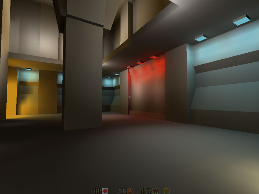
Quake2 was the first engine released with native support for hardware accelerated rendering. He demonstrated undeniable improvements due to bilinear texture filtering, increased multitexturing, and 24-bit color mixing.
From the user's point of view, the hardware accelerated version provided the following improvements:
- Bilinear filtering
- Color lighting
- 30% higher frame rate at high resolutions
I can not refrain from quoting from “Masters of Doom” about how John Romero first saw the color lighting [app. Lane: before starting work on Quake 2, he already left id Software and created his own company Ion Storm] :
id [...].
, Quake II. , : ! , . , , . , . , Softdisk, Dangerous Dave in Copyright Infringement [. .: 1990 PC ] .
« », — . .
This feature has had a strong influence on the development of Daikatana.
In terms of code, the renderer is 50% smaller than the software renderer (see "Code Statistics" at the bottom of the page). This meant that developers needed less work. Also, this implementation was much simpler and more elegant than the software / assembly-optimized version:
- Z-buffer eliminated the stack of active polygons (this dependence on a fast Z-buffer led to problems when developing VQuake for V2200
- The high speed of the rasterizer chips in combination with the speed of the Z-buffer RAM made the task of zero redrawing unnecessary.
- The built-in procedure of line-by-line construction of the image eliminated the need for a global edge table and a table of active edges.
- The illumination maps were filtered in the video processor (and in RGB instead of grayscale): these calculations did not fall into the CPU at all.
After all, the OpenGL renderer is more a resource manager than a renderer: it passes vertices, loads a satin of lightmaps on the fly, and assigns texture states.
An interesting fact: the Quake2 frame usually contains 600-900 polygons each: a striking difference from the millions of polygons in any modern engine.
Global code architecture
The rendering phase is very simple and I will not discuss it in detail, because it is almost identical to software rendering:
R_RenderView { R_PushDlights // , R_SetupFrame R_SetFrustum R_SetupGL // GL_MODELVIEW GL_PROJECTION R_MarkLeaves // PVS R_DrawWorld // , BoundingBox { } R_DrawEntitiesOnList // R_RenderDlights // R_DrawParticles // R_DrawAlphaSurfaces // - R_Flash // ( ....) } All stages are clearly shown in the video, in which the engine is "slowed down":
Visualization order:
- World.
- Entities (in Quake2, they are called "alias").
- Particles
- Translucent surfaces.
- Fullscreen post effects.
The main complexity of the code arises from different paths, depending on whether the video card supports multi-texturing and whether vertex group rendering is enabled. For example, if the multi-texturing is supported,
DrawTextureChainsand R_BlendLightmapsin the following piece of code is not doing anything and just confusing when reading the code: R_DrawWorld { // , 100% () R_RecursiveWorldNode // , { // PVS BBox/ // ! // : GL_RenderLightmappedPoly { if ( is_dynamic ) { } else { } } } // ( ) DrawTextureChains // , bindTexture. { for ( i = 0, image=gltextures ; i<numgltextures ; i++,image++) for ( ; s ; s=s->texturechain) R_RenderBrushPoly (s) { } } // ( : ) R_BlendLightmaps { // // if ( gl_dynamic->value ) { LM_InitBlock GL_Bind for ( surf = gl_lms.lightmap_surfaces[0]; surf != 0; surf = surf->lightmapchain ) { // . , , } } } R_DrawSkyBox R_DrawTriangleOutlines } World visualization
Level rendering is done in
R_DrawWorld. A vertex has five attributes:- Position.
- Color texture identifier.
- Coordinates color texture.
- The texture ID of the static lightmap.
- The coordinates of the static map of the lighting.
In the OpenGL renderer there is no “Surface”: colors and lighting map are combined on the fly and never cached. If the video card supports multitexturing, then only one pass is needed, indicating the texture identifier and its coordinates:
- The color texture is tied to the OpenGL GL_TEXTURE0 state.
- The lightmap texture is tied to the OpenGL GL_TEXTURE1 state.
- Transmitted vertices with the coordinates of the color texture and lighting map texture.
If the video card does NOT support multi-texturing, then two passes are performed:
- Mixing is turned off.
- The color texture is tied to the OpenGL GL_TEXTURE0 state.
- Vertices are sent with color texture coordinates.
- Mixing is turned on.
- The lightmap texture is tied to the OpenGL GL_TEXTURE0 state.
- Transmitted vertices with the coordinates of the lighting map texture.
Texture Management
Since all rasterization is performed in the video processor, at the beginning of the level all textures should be loaded into the video memory:
- Color textures
- Pre-calculated lighting map textures
Using the OpenGL gDEBugger debugger, you can easily dig into the memory of a video processor and get statistics:

As we can see, each color texture has its own texture identifier (textureID). Static lighting maps are loaded as a texture atlas (called a “block” in quake2) in the following form:

Why is the color texture in a separate texture if the lighting maps are collected in a texture atlas?
The reason is the optimization of the chains of textures :
If you want to increase performance when working with a video processor, then you need to strive for it to change its state as little as possible. This is especially true for texture binding (
glBindTexture). Here is a bad example: for(i=0 ; i < polys.num ; i++) { glBindTexture(polys[i].textureColorID , GL_TEXTURE0); glBindTexture(polys[i].textureLightMapID , GL_TEXTURE1); RenderPoly(polys[i].vertices); } If each polygon has a color texture and a lighting map texture, then there is little that can be done, but Quake2 collects its lighting maps into atlases, which can be easily grouped by identifier. Therefore, polygons are not rendered in the order returned from BSP. Instead, they are grouped into texture chains based on which atlas of lightmap textures they belong to:
glBindTexture(polys[textureChain[0]].textureLightMapID , GL_TEXTURE1); for(i=0 ; i < textureChain.num ; i++) { glBindTexture(polys[textureChain[i]].textureColorID , GL_TEXTURE0); RenderPoly(polys[textureChain[i]].vertices); } The video below shows the process of rendering “chains of textures”: polygons are rendered not depending on the distance, but on the basis of a block of lighting maps to which they belong:
Note: to achieve constant translucency, only completely opaque polygons fall into the texture chain, and translucent polygons are still rendered back to front.
Dynamic lighting
At the very beginning of the visualization phase, all polygons are marked to show that they are affected by dynamic lighting (
R_PushDlights). Therefore, a pre-calculated static lighting map is not used. Instead, a new irradiance map is generated, combining a static irradiance map with the addition of light projected onto the plane of the polygon ( R_BuildLightMap).Since the lighting map has a maximum size of 17x17, the phase of generating a dynamic lighting map is not very expensive, but loading changes into the video processor using a
qglTexSubImage2D very slow one.To store all dynamic lighting maps, a block of lighting maps of 128x128 is used, its id = 1024. See the “Lighting Map Management” section for an explanation of how all dynamic lighting maps are combined on the fly into a texture atlas.
1. The initial state of the dynamic lighting unit. 2. After the first frame. 3. After ten frames.
Note: If the dynamic lighting map is full, group rendering is performed. The rover tracks whether the allocated space has been cleared and the generation of dynamic lighting maps is resumed.
Lighting map management
As I said earlier, in the OpenGL version of the renderer there is no concept of "surface" ("surface"). The lighting map and color texture are combined on the fly and are NOT cached.
The static lighting maps are loaded into the video memory, they are still stored in RAM: if the polygon is affected by dynamic lighting, a new lighting map is generated, combining a static lighting map with the light projected on it. The dynamic lightmap is then loaded into textureId = 1024 and used for texturing.
Texture atlases are called “blocks” (“Block”) in Quake2, consist of 128x128 texels and are controlled by three functions:
LM_InitBlock: Reset tracking of memory consumption by block.LM_UploadBlock: Download or update texture contents.LM_AllocBlock: Find a suitable place to store your lighting map.
The video below shows how the lighting maps are combined into blocks. Here the engine plays in "Tetris": scans from left to right and remembers where the lighting map will fit completely in the highest coordinate of the image.
The algorithm should pay attention: rover (
int gl_lms.allocated[BLOCK_WIDTH]) tracks across the entire width, which height each column of pixels occupied. // "best" "bestHeight" // "best2" "tentativeHeight" static qboolean LM_AllocBlock (int w, int h, int *x, int *y) { int i, j; int best, best2; //FCS: best = BLOCK_HEIGHT; for (i=0 ; i<BLOCK_WIDTH-w ; i++) { best2 = 0; for (j=0 ; j<w ; j++) { if (gl_lms.allocated[i+j] >= best) break; if (gl_lms.allocated[i+j] > best2) best2 = gl_lms.allocated[i+j]; } if (j == w) { // *x = i; *y = best = best2; } } if (best + h > BLOCK_HEIGHT) return false; for (i=0 ; i<w ; i++) gl_lms.allocated[*x + i] = best + h; return true; } Note: the rover design pattern (“rover”) is very elegant and is also used in the system of memory caching of the surfaces of the software renderer.
Pixel fill rate and rendering passes
As can be seen from the following video, redrawing can be quite significant:
In the worst case, a pixel can be overwritten 3-4 times (not counting redrawing):
- World: 1-2 passes (depending on multitexturing support).
- Particle mixing: 1 pass.
- Post-effect mixing: 1 pass.
GL_LINEAR
Bilinear filtering worked well with color textures, but really blossomed when filtering lighting maps:
It was:
It became:
And now all together:

1. Texture: dynamic / static lighting map.

2. Texture: color.

3. Mixing result: one or two passes.
Entity visualization
Entities are rendered in groups: vertices, texture coordinates, and color array pointers are collected and sent using
glArrayElement.Before rendering, LERP is performed for the vertices of all entities to smooth the animation (in Quake1, only keyframes were used).
Gouraud's lighting model is used: an array of colors is intercepted by Quake2 to store the lighting value. Before rendering, the light value is calculated for each vertex and stored in an array of colors. The value of this array is interpolated in the video processor and a good result is obtained with Guro lighting.
R_DrawEntitiesOnList { if (!r_drawentities->value) return; // for (i=0 ; i < r_newrefdef.num_entities ; i++) { R_DrawAliasModel { R_LightPoint /// GL_Bind(skin->texnum); // GL_DrawAliasFrameLerp() // { GL_LerpVerts // LERP // , colorArray for ( i = 0; i < paliashdr->num_xyz; i++ ) { } qglLockArraysEXT qglArrayElement // ! qglUnlockArraysEXT } } } // for (i=0 ; i < r_newrefdef.num_entities ; i++) { R_DrawAliasModel { [...] } } } Cutting off the rear edges is performed in a video processor (well, since the tessellation and lighting were performed at that time in the CPU, I think we can say that it was performed at the driver stage).
Note: to accelerate calculations, the direction of light has always been taken to be the same (
{-1, 0, 0}), but this is not reflected in the engine. The illumination color is accurate and is selected according to the current polygon on which the entity is based.This is very clearly seen in the screenshot below, where the light and shade are in the same direction, despite the incorrect definition of the light source.
Note: Of course, this system is not always perfect, the shadow is emitted into the void, and the edges overwrite each other, leading to different levels of shadows, but this is still pretty impressive for 1997.
More about shadows:
Many do not know that Quake2 was able to calculate the approximate shadows of entities. Although this feature is disabled by default, it can be enabled with a command
gl_shadows 1.The shadow is always directed in one direction (does not depend on the nearest source of light), the faces are projected onto the plane of the essence level. In the code, it
R_DrawAliasModelgenerates a vector shadevectorused GL_DrawAliasShadowto project the faces onto the plane of the entity level.Entity Visualization Lighting: Discretization Trick
, / … .
float r_avertexnormal_dots[SHADEDOT_QUANT][256] , SHADEDOT_QUANT =16.: : {-1,0,0}.
16 , Y.
16 256 . MD2 — . X,Y,Z 256 .
-
r_avertexnormal_dots16x256 size. Since the normal index cannot be interpolated during the animation process, the closest normal index is used for the keyframe.More on this: http://www.quake-1.com/docs/quakesrc.org/97.html ( mirror ).
Good old OpenGL ...
glGenTextures?!:
openGL- textureID
glGenTextures . Quake2 . 0, 1024, 1025 1036.Immediate mode:
ImmediateMode. (
glVertex3fv glTexCoord2f ) ( , ).(, )
glEnableClientState (GL_VERTEX_ARRAY) . , glVertexPointer glColorPointerused to transmit the value of the illumination calculated in the CPU.Multitexturing:
The code is complicated by the fact that it seeks to adapt to the equipment that supports and does not support the new technology ... multitexturing.
No use
GL_LIGHTING:Since all calculations were performed in the CPU (generating textures for the world and the value of the vertex illumination for entities), there are no traces in the code
GL_LIGHTING.Since OpenGL 1.0 still performed Gouraud shading (interpolating colors between vertices) instead of Phong shading (where normals are interpolated for real “pixel-by-pixel illumination”), using
GL_LIGHTINGit would look bad for the world because it would require creating vertices on the fly.It could be applied to entities, but at the same time, we would have to send vertex normal vectors. This seems to be considered unsuitable, therefore the calculation of the illumination values is performed in the CPU. The light value is transferred from the color array, the values are interpolated to the CPU to get Gouro shading.
Fullscreen post effects
The palette-based software renderer performed elegant full color mixing of the palette and additional gamma correction using a lookup table. But the OpenGL-version is not necessary, and this can be seen on the example of the “brute force” method in
R_Flash:Problem: do you need to make the screen a little more red?
Solution: just draw a huge red rectangle GL_QUAD on the whole screen with alpha channel mixing turned on. Is done.
Note: the server controlled the client in the same way as the software renderer: if the server needed to perform full-screen color mixing for the post-effect, it simply assigned the value of the
float player_state_t.blend[4]RGBA variable . The value of the variable is then transmitted through the quake2 kernel over the network and sent to the renderer DLL.Profiling
Visual Studio 2008 Team Profiler is just wonderful, that's what it turned out for OpenGL Quake2:

No wonder: most of the time is spent on OpenGL-driver NVidia and Win32 (
nvoglv32.dlland opengl32.dll), only about 30%. The visualization is performed in the video processor, but a lot of time is spent on a multiple call of the immediate mode methods, as well as on copying data from RAM to the video memory.The following are the renderer module (
ref_gl.dll23%) and the quake2 kernel ( quake2.exe15%).Even in spite of the fact that the engine actively uses malloc, we see that time (
MSVCR90D.dlland msvcrt.dll) is almost not wasted on it . The time spent on the game logic ( gamex86.dll) is also irrelevant .Unexpected amount of time spent on directX (
dsound.dll) sound library : 12% of total time.Let's take a closer look at the OpenGL Quake2 renderer dll:

- Most of the time is spent on rendering the world (
R_RecurseiveWorldNode). - Almost the same - for rendering enemies (alias models): (
GL_DrawAliasFrameLerp2.5%). The costs are quite high, despite the fact that the dot product is calculated in advance. - The generation of lighting maps (when dynamic lighting prevents the use of a previously computed static lighting map) also takes 2.5% of the time (
GL_RenderLightMappedPoly).
In general, the OpenGL dll is well balanced, there are NO obvious bottlenecks.
Code statistics
An analysis of the Cloc code shows that there are a total of 7,265 lines of code.
$ cloc ref_gl 17 text files. 17 unique files. 1 file ignored. http://cloc.sourceforge.net v 1.53 T=1.0 s (16.0 files/s, 10602.0 lines/s) ------------------------------------------------------------------------------- Language files blank comment code ------------------------------------------------------------------------------- C 9 1522 1403 6201 C/C++ Header 6 237 175 1062 Teamcenter def 1 0 0 2 ------------------------------------------------------------------------------- SUM: 16 1759 1578 7265 ------------------------------------------------------------------------------- Compared to the software renderer, the difference is astounding: 50% less code, WITHOUT assembler optimization, while the speed is 30% higher and there is color lighting and bilinear filtering. It is easy to understand why id Software did not bother with the software renderer for Quake3.
Source: https://habr.com/ru/post/328128/
All Articles