Working with Dunno - Proactive Reading Technologies and Hybrid Storage

One way to improve performance and reduce latency in storage systems (DSS) is to use algorithms that analyze incoming traffic.

On the one hand, it seems that requests to the storage system are highly dependent on the user and, accordingly, little predictable, but in fact it is not.

The morning of almost every person is the same: we wake up, dress, wash our face, have breakfast, go to work. The working day, depending on the profession, is different for everyone. Also, the storage load is the same every day, but the work day depends on where the storage is used and what its typical load (workload) is.
')
In order to more clearly present our ideas, we used the images of characters from children's stories about Nikolai Nosov. In this article, the main actors will be Dunno (random reading) and Znayka (sequential reading).


Random read (random read) - Dunno . C Dunno nobody wants to deal. His behavior defies logic. Although some algorithms still try to predict its behavior, for example, sophisticated algorithms of prefetching from memory type C-Miner (it will be discussed in more detail below). These are machine learning algorithms - it means that they are demanding on storage resources and are not always successful, but due to the enormous development of computing power of processors, more and more will be used in the future.

If only Dunnies come to the storage system, then the best solution would be SSD-based storage systems (All-Flash Storage).

Sequential reading (sequential read) - Znayka . Strict, pedantic and predictable. Due to this behavior, it can be considered the best friend for storage. There are read-ahead algorithms that can work well with Znayka, they place the necessary data in RAM in advance, reducing the latency of the request to a minimum.

Blender effect

Sequential reading is predictable, but the reader may argue: “But what about the blender effect <fig. 1>, which makes consecutive requests random as a result of mixing traffic? ".

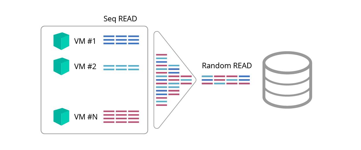
Fig. 1. Blender effect

Do knowledgeable as a result of such confusion will become Dunno?

An advanced read algorithm and a detector that can identify different types of queries come to the aid of Znayka.

Read ahead

One of the main optimization methods designed to reduce access time and increase throughput is the use of read ahead technology. The technology allows, based on the data already requested, to predict what data will be requested next, and transfer them from slower media (for example, from hard drives) to faster (for example, RAM and solid-state drives) before these data are accessed. (Fig. 2).

In most cases, read ahead is used for sequential operations.



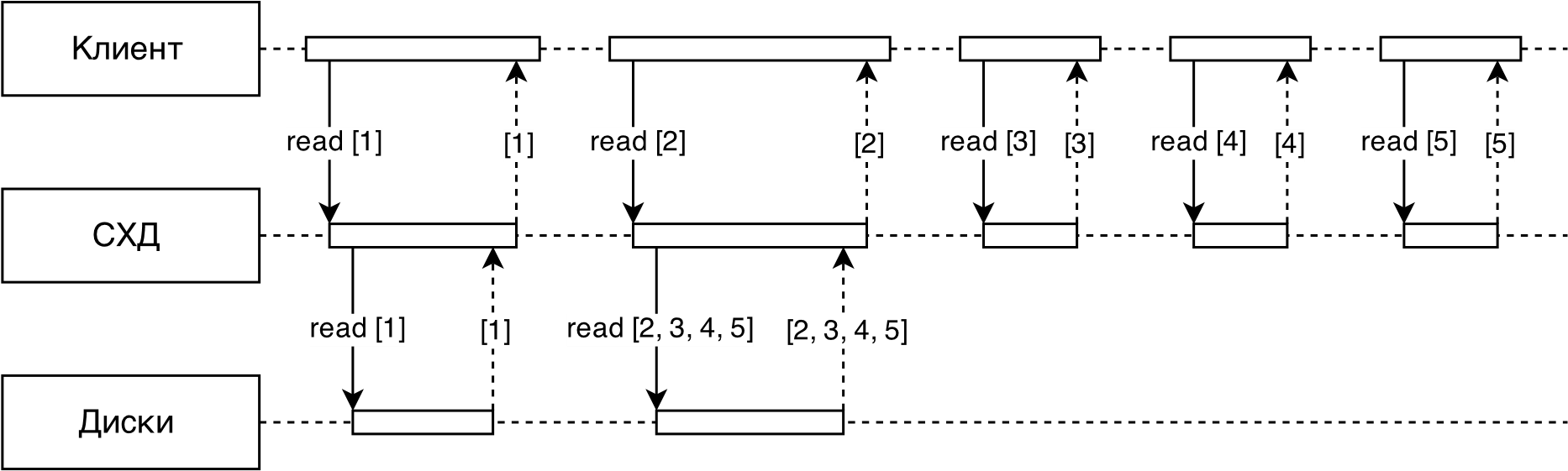
Fig. 2. Proactive reading

The work of the read-ahead algorithm is divided into two stages:

1. detection of sequential read requests in the stream of all requests;
2. deciding whether to read data in advance and read volumes.

Detector Implementation in RAIDIX

The proactive read algorithm in RAIDIX is based on the concept of ranges corresponding to the coherent intervals of the address space.

Ranges are indicated by pairs ( $$$lba_i, len_i$), which corresponds to the address and length of the request, and are sorted by $$$lba$. They are divided into random, the length of which is less than a certain threshold, and consistent. Simultaneously tracked to $$$N$random ranges and up $$$M$consecutive.

The detector algorithm works as follows:

1. For each incoming read request, the nearest ranges are searched within the strideRange radius.
1.1. If there are none, a new random range is created with the address and length corresponding to the characteristics of the request. However, one of the existing ranges can be superseded by LRU.
1.2. If one range is found, the query is added to it with an interval extension. A random range can be converted to a serial one.
1.3. If there were two ranges (left and right), they are combined into one. The resulting range of this operation can also be converted to serial.
2. If the request is in the sequential range, a prefetch reading can be made for this range.

The read ahead parameter may vary depending on the flow rate and block size.

Figure 3 shows a schematic of an adaptive read-ahead algorithm implemented in RAIDIX.

Fig.3. Prefetch schema

All requests to the storage system from the client first fall into the detector, its task is to select sequential streams (to distinguish sequential requests from random ones).

Further, for each sequential flow, its speed is determined $$$v$and size $$$len$- the average size of the request in the stream (usually in the stream all requests of the same size).

Each thread is mapped to the read ahead parameter. $$$m = f (v, len)$.

Thus, with the aid of the read-ahead algorithm, we cope with the “I / O blender” effect and for sequential requests we guarantee throughput and latency comparable to the parameters of the RAM.

Thus Znayka defeats Dunno!

Random read performance

How can you improve the performance of random reading?

For these purposes, the developers Vintik and Shpuntik propose to use faster media, namely SSD and a hybrid solution (tearing or SSD cache).



You can also use a random query accelerator — the C-Miner read-ahead algorithm.

The main objective of all these methods is to put Dunno on a “fast” car :-) The problem is that you must be able to drive a car, and Dunno is too unpredictable.

C-Miner

One of the most interesting algorithms used for read-ahead with random requests is C-Miner, based on the search for correlations between the addresses of sequentially requested data blocks.

This algorithm detects semantic links between queries, such as querying file system metadata before reading the corresponding files or searching for a record in the DBMS index.

C-Miner operation consists of the following steps:

1. A sequence of I / O request addresses reveals repeated short subsequences bounded by a window of some size.
2. From the resulting subsequences, suffixes are extracted, which are then combined according to the frequency of occurrence.
3. Based on the extracted suffixes and chains of suffixes, rules of the form {a → b, a → c, b → c, ab → c} are generated, which describe which data blocks are preceded by requests for addresses from the correlating domain.
4. The rules obtained are ranked according to their reliability.

The C-Miner algorithm is well suited for storage systems, in which data is rarely updated, but is often requested in small portions. This use case allows you to create a set of rules that will not become obsolete for a long time, and also will not slow down the execution of the first queries (appeared before the rules were created).

In the classical implementation, there are often many rules with low reliability. In this connection, read-ahead algorithms do a rather poor job with random queries. It is much more efficient to use a hybrid solution, in which the most popular queries fall on more efficient drives, for example, SSD or NVME disks.

SSD cache or SSD-tiring?

The question arises, which technology is better to choose: SSD-cache or SSD-tearing? A detailed analysis of the workload will help answer this question.

The SSD cache is schematically depicted in Figure 4. Here, requests first fall into RAM, and then, depending on the type of request, can be pushed into the SSD cache or into main memory.

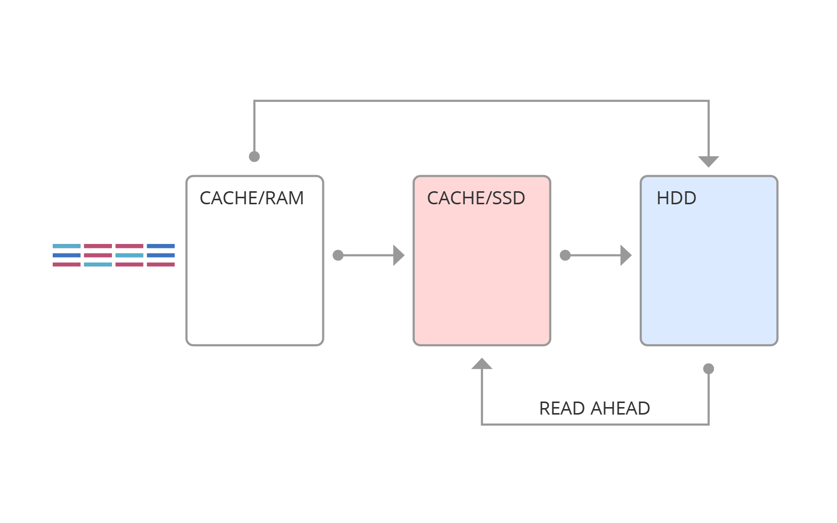
Fig. 4. SSD cache

SSD-tiring has a different structure (Fig. 5). With the tearing, the statistics of hot areas are kept, and at fixed points in time, the hot data is transferred to faster media.

Fig. 5. SSD-Tiring

The main difference between SSD-cache and SSD-tiring is that the data in the tearing are not duplicated, unlike SSD-cache, in which the “hot” data is stored both in the cache and on the disk.

The table below shows some selection criteria for a solution.

	Tiring	Cache
Research method	Predicting future values	Identifying Locality in Data
Workload	Predictable. Slightly changing	Dynamic, unpredictable. Requires instant reaction
Data	Not duplicated (disk)	Duplicate (buffer)
Data migration	Offline-algorithm, relocation window (relocation window). There is a time parameter for moving data	Online algorithm, data is pushed out and get into the cache on the fly.
Research methods	Regression models, prediction models, long-term memory	Short-term memory, crowding algorithms
Interaction	HDD-SSD	RAM-SSD, interaction with SSD through read-ahead algorithms
Block	Large (for example, 256 MB)	Small (for example, 64 KB)
Algorithm	Function depending on the transfer time and the statistical characteristics of memory addresses	Algorithms for crowding out and filling
Read / write	Random reading	Any requests, including write requests, with the exception of sequential reads (in most cases)
Motto	The harder the better	The simpler the better
Manual transfer of necessary data	Available	Not possible - contrary to the logic of the cache

The basis of any hybrid solution, one way or another, is the prediction of future load. In the tearing, we are trying to predict the future from the past, in the SSD cache we believe that the likelihood of using recent and frequency queries is higher than that used for a long time and low frequencies. In any case, the basis of the algorithms is the study of the "past" load. If the nature of the load changes, for example, a new application starts to work, then it takes time for the algorithms to adapt to the changes.

Dunno is not to blame (his character is so random) that the hybrid solution is poorly managed in an unknown new area!



But even with the right "prediction", the performance of the hybrid solution will be low (well below the maximum performance that an SSD drive can deliver).

Why? The answer is below.

How much IOPS to expect from SSD cache?

Suppose we have a 2TB SSD cache and a cached volume is 10TB. We know that some process randomly reads the entire volume with a uniform distribution. We also know that from the SSD cache we can read at a speed of 200K IOPS, and from a non-cached area at a speed of 3K IOPS. Suppose that the cache is already full, and it contains 2 out of 10 TB read. How many IOPS will we get? The obvious answer comes to mind: 200K * 0.2 + 3K * 0.8 = 42.4K. But is it really that simple?

Let's try to figure it out by applying a bit of math. Our calculations deviate somewhat from real practice, but are quite acceptable for evaluation purposes.

DANO:

Let x% of read data (or even requests) lie (processed) in the SSD cache.
We assume that the SSD cache processes requests with the speed u IOPS. And requests going to the HDD are processed at a speed of v IOPS.

DECISION:

First, consider the case when iodepth (depth of the request queue) = 1.
Take the size of the entire readable space for 1. Then the share of data (requests) that are (processed) in the cache will be x / 100.

Let 1 second processed $$$I$requests. Then from them $$$I * x / 100$cached and the rest $$$I * (100-x) / 100$go to HDD. This is true due to the fact that reading occurs with a uniform distribution.

Take for $$$t_1$the total time spent on those requests that went to the SSD, but for $$$t_2$time spent on HDD requests.

Since now we are considering only one second, $$$t_1 + t_2 = 1$(s)

We have the following equality (1): $$$u * t_1 + v * t_2 = I$. Using units of measure: IOPS * s + IOPS * s = IO.

We also have the following (2): $$$I * x / 100 = t_1 * u$. Express I: $$$I = t1 * u * 100 / x$.

Substitute in (1) obtained from (2) I: $$$u * t_1 + v * t_2 = t_1 * u * 100 / x$. Express $$$t_1$considering that $$$t_2 = 1 - t_1: t_1 = v / (u * 100 / x + v - u)$.

Know $$$t_1$then we know and $$$t_2: t_2 = 1- v / (u * 100 / x + v - u)$.

Got times $$$t_1$and $$$t_2$, now we can substitute them in (1): $$$I = u * v / (u * 100 / x + v - u) + v - v * v / (u * 100 / x + v - u)$.

Simplify equality: $$$I = 100 * u * v / (v * x + u * (100 - x))$.

Fine! Now we know the number of IOPS with iodepth = 1.
What happens when iodepth> 1? These calculations will be incorrect, or rather, not quite true. You can try to consider several parallel streams, for each of which iodepth = 1, or come up with a different method, however, with sufficient test duration, these inaccuracies will smooth out, and the picture will be the same as with iodepth = 1. The result will still reflect the real picture .

So, answering the question “how much will IOPS be?”, We apply the formula:

$$

$$I (x, u, v) = 100 * u * v / (v * x + u * (100 - x)).$$

Generalization

And what if we do not have a uniform distribution, but some closer to life?
Take, for example, the Pareto distribution (80/20 rule - 80% of requests go to 20% of the “hottest” data).

In this case, the resulting formula also works, since we have not relied anywhere on the size of the space and the size of the SSD. It is only important for us to know how many% of requests (in this case, namely requests!) Will be processed in the SSD.

If the size of the SSD cache is 20% of the total readable space and accommodates these 20% of the “hottest” data, then 80% of the requests will go to the SSD. Then, according to the formula I (80, 200000, 3000) ≈ 14150 IOPS. Yes, most likely, it is less than you thought.

Let's build the graph I (x) with u = 200000, v = 3000.



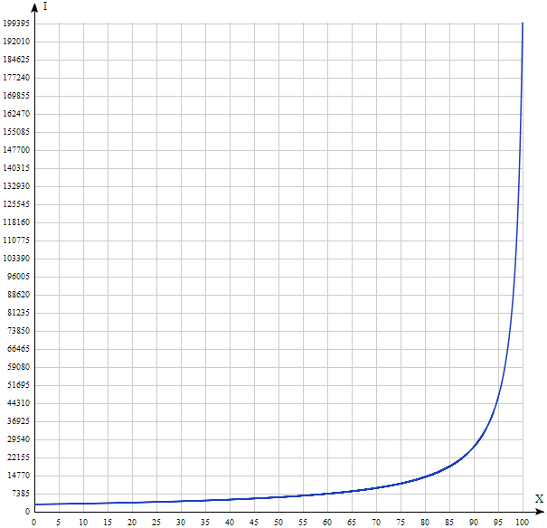
The result is significantly different from the intuitive. Thus, handing Dunno the keys to a fast car, we can not always accelerate system performance. As can be seen from the graph above, only the All-Flash solution (where all the drives are solid-state) can really speed up random reading to the maximum “squeezed out” from the SSD disk. It is not Dunno that is to blame for this, and, of course, not the developers of data storage systems, but simple mathematics.