Explanation of Neural Turing Machines
I found that the overwhelming majority of online information about research in the field of artificial intelligence is divided into two categories: the first tells about the achievements of a lay audience, and the second to other researchers. I have not found a good resource for people with technical education who are not familiar with more advanced concepts and are looking for information to fill in the gaps. This is my attempt to fill this void by providing accessible, but at the same time (relatively) detailed explanations. Here I will explain Graves, Wayne, and Danikey’s (2014) scientific article on Turing Neural Machines (NTM).
Initially, I was not going to talk about this article, but I could not understand another interesting article I was going to talk about. It was about the NTM modification, so I decided to make sure I fully understand NTM before moving on. After verifying this, I had the feeling that that second article was not very suitable for explanation, but the original work on NTM was very well written, and I strongly recommend it to be read.
During the first thirty years of artificial intelligence research, neural networks were considered mostly unpromising. From the 1950s to the late 1980s, the symbolic approach dominated AI. He assumed that the work of information processing systems like the human brain can be understood through manipulations with the symbols, structures, and rules of processing these symbols and structures. Only in 1986 appeared a serious alternative to symbolic AI; its authors used the term "parallel distributed processing" (Parallel Distributed Processing), but today the term " connectionism " is more often used. You might not have heard of such an approach, but you probably heard about one of the most famous connection modeling modeling techniques - artificial neural networks.
Critics have put forward two arguments against the fact that neural networks will help us better understand intelligence. Firstly, neural networks with a fixed size of input data, apparently, are not able to solve problems with input data of variable size. Secondly, neural networks seem to be unable to bind values to a specific location in data structures. The ability to write and read from memory is critical in both information processing systems that are available for study: in the brain and computers. In that case, what can be answered to these two arguments?
')
The first argument was refuted with the creation of recurrent neural networks (RNN). They can process variable-size input without needing to modify or add a time component to the processing procedure — when translating a sentence or recognizing handwritten text, RNN repeatedly receives input data of a fixed size as many times as required. In his scientific article, Graves et al. Tries to refute the second argument, giving the neural network access to external memory and the ability to learn how to use it. They called their system the Neural Turing Machine (NTM) .
For specialists in computer theory, the need for a memory system is obvious. Computers have tremendously improved over the past half century, but they still consist of three components: memory, control logic, and arithmetic / logic operations. There are also biological evidence points to the benefits of a memory system for quickly storing and retrieving information. Such a memory system is called working memory , and the article on NTM refers to several earlier works that studied working memory from the point of view of computational neuroscience.
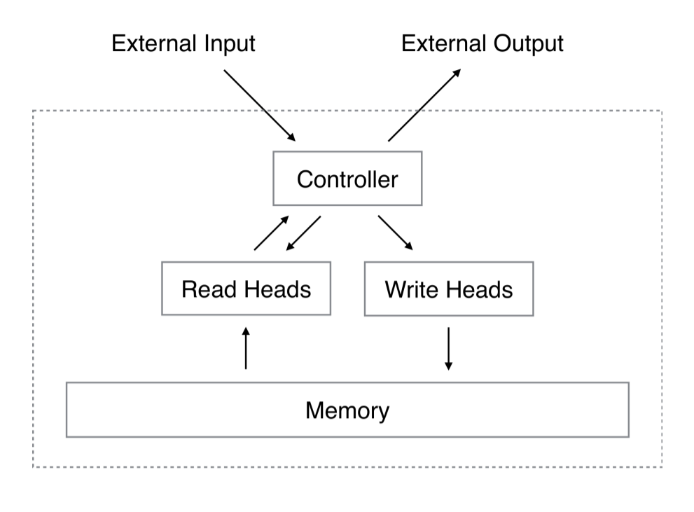
The NTM schematic diagram includes a neural network called a controller , a 2D matrix (memory bank), and a memory matrix or ordinary memory . At each time step, the neural network receives some data from the outside world and sends some output to the outside world. However, the neural network also has the ability to read information from individual memory cells and the ability to write to individual memory cells. Graves et al. Drew inspiration from the traditional Turing machine and used the term “head” to describe memory cell operations. In the diagram below, the dashed line restricts parts of the architecture that are “inside” the system in relation to the outside world.
But there is a catch. Suppose we index the memory by specifying a row and column, as in a regular matrix. We would like to train our neural network using the error back-propagation method and our favorite optimization method (for example, the stochastic gradient method), but how to get a certain index gradient? Will not work. Instead, the controller performs read and write operations as part of “fuzzy” operations that interact with all the elements in memory to one degree or another. The controller will calculate the weights for the memory cells, which will allow it to determine the memory cells in a differentiated way. Next, I will explain how these weight vectors are generated, and then how they are used (it is easier to understand the system).
Take the memory matrix with rows and items in a row with time as . In order to read (and write), a certain attention mechanism is required, which determines where the head should read data from. The mechanism of attention will be normalized in length. (length- ) weight vector . We will talk about the individual elements of the weight vector as . By "rationing" authors imply the observance of the following two limitations:
The reading head will return the normalized length (length- ) vector which is a linear combination of strings of memory scaled by weight vector:
Writing is a bit more complicated than reading because it involves two separate steps: erasing, then adding. To erase old data, the recording head needs a new vector, this is length- erase vector in addition to our length- normalized weight vector . The erase vector is used in conjunction with a weight vector to determine which elements in the line should be removed, left unchanged, or something in between. If the weight vector points to a line, and the erasing vector indicates an erase element, then the element in this line will be erased.
After conversion at the recording head uses length- adding vector to complete the write operation.
Creating such weight vectors to determine where to read and write data is not easy, I would present this process in four stages. At each stage, an intermediate weight vector is generated, which is passed to the next stage. The goal of the first stage is to generate a weight vector based on how close each line in memory is to length. vector released by the controller. We will call this intermediate weight vector weight vector content. Other parameter I'll explain now.
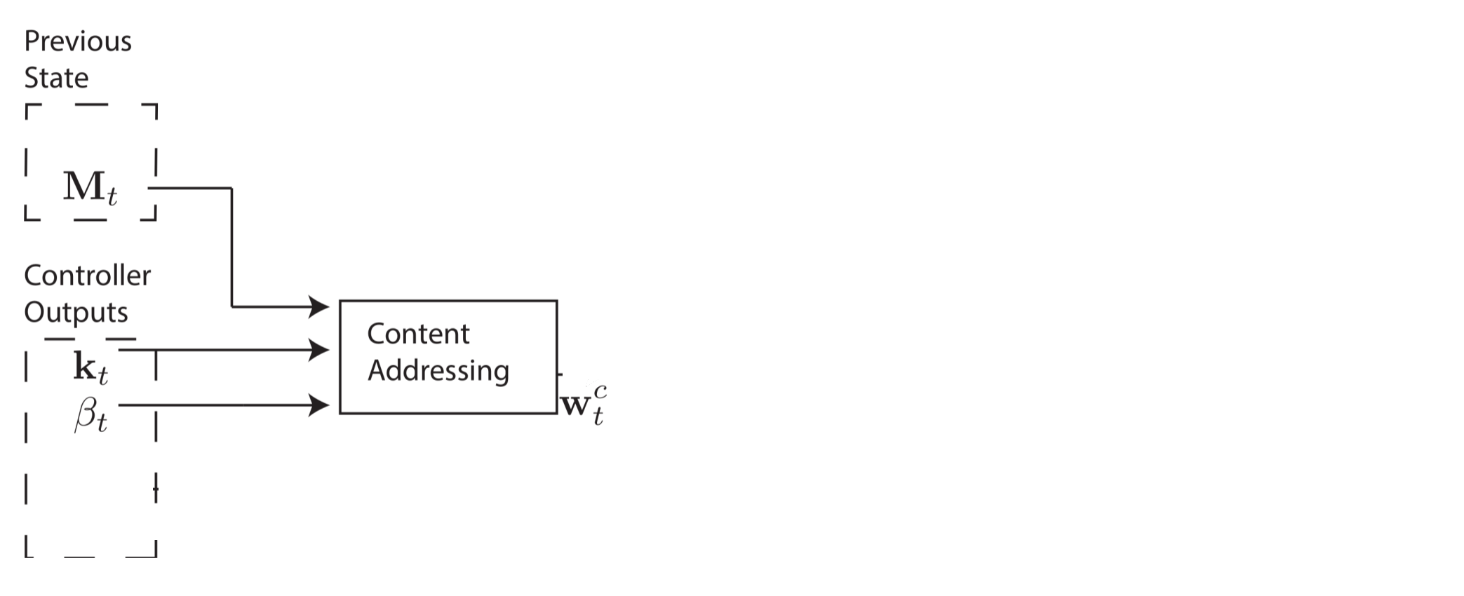
The weight vector of the content allows the controller to select values that are similar to already known values, which is called content addressing. For each head, the controller produces a key vector. which is compared with each line using a measure of similarity. In this paper, the authors use the cosine measure of similarity, which is defined as follows:
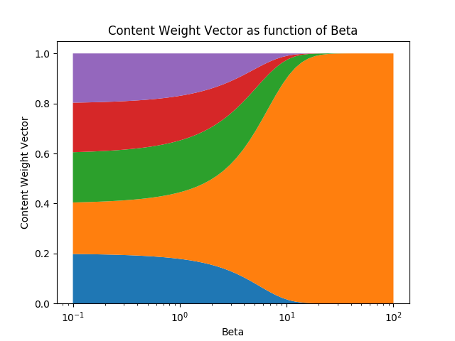
Positive scalar parameter Which is called key strength is used to determine how concentrated the weight vector of the content should be. For small values of beta, the weight vector will be blurred, and for large values of beta, the weight vector will be concentrated on the most similar line in memory. For visualization, if the key and the memory matrix produce a similarity vector
Weight vector content can be calculated as follows:
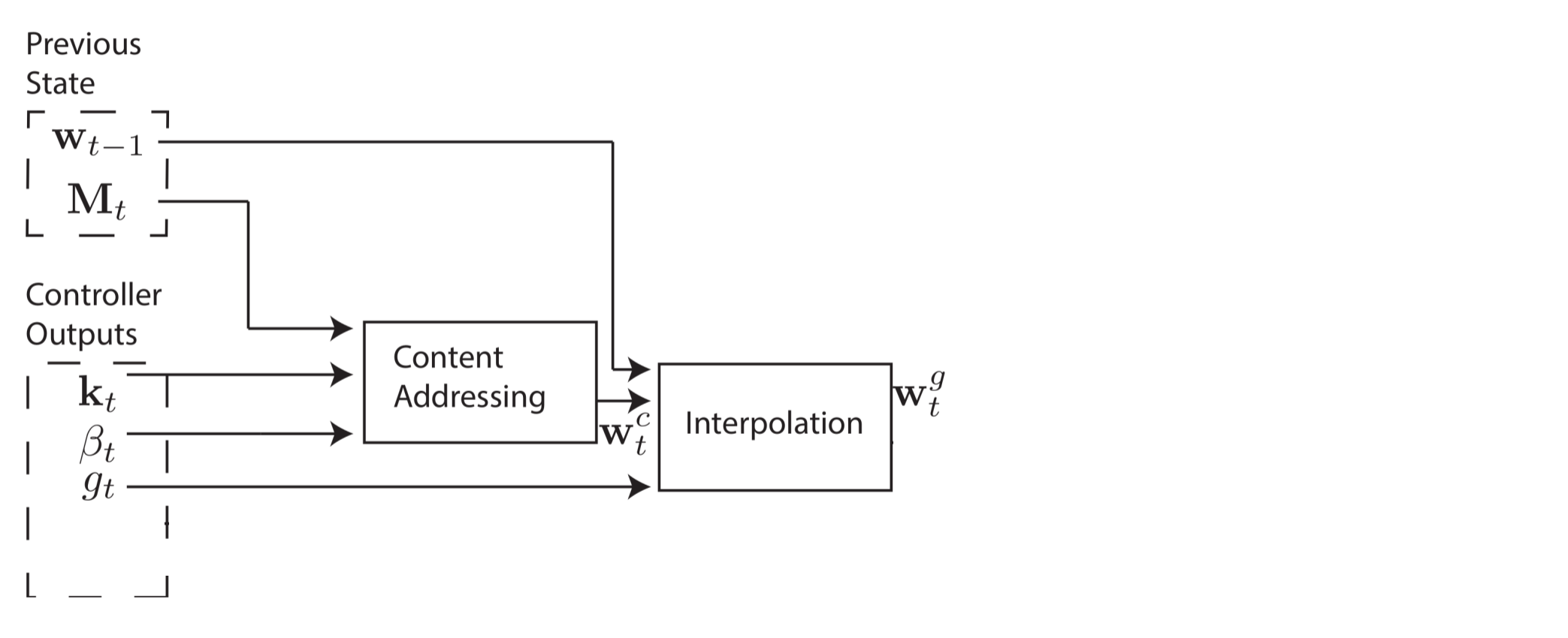
However, in some cases we may want to read from specific memory cells, rather than read specific values in memory. For example, the authors show the function . In this case, we do not care about the specific values of x and y, only that they are constantly read from the same cells in memory. This is called cell addressing, and for its implementation we need three more steps. In the second stage, the scalar parameter which is called the interpolation gate, mixes the weight vector of the content with the weight vector of the previous time step for the production of valve weight vector . This allows the system to understand when to use (or ignore) content addressing.
We would like the controller to shift the focus to other lines. Suppose that one of the system parameters is limited to the range of allowable offsets. For example, the head's attention may shift forward one line (+1), remain unchanged (0), or move backward (-1) a line. Perform shifts by module so that moving forward from the bottom row of memory moves the head's attention to the top line, just as moving backward from the top line moves the head's attention to the bottom line. After interpolation, each head produces a normalized shift weighting. and the following convolutional movement occurs to calculate the weight of the shift .
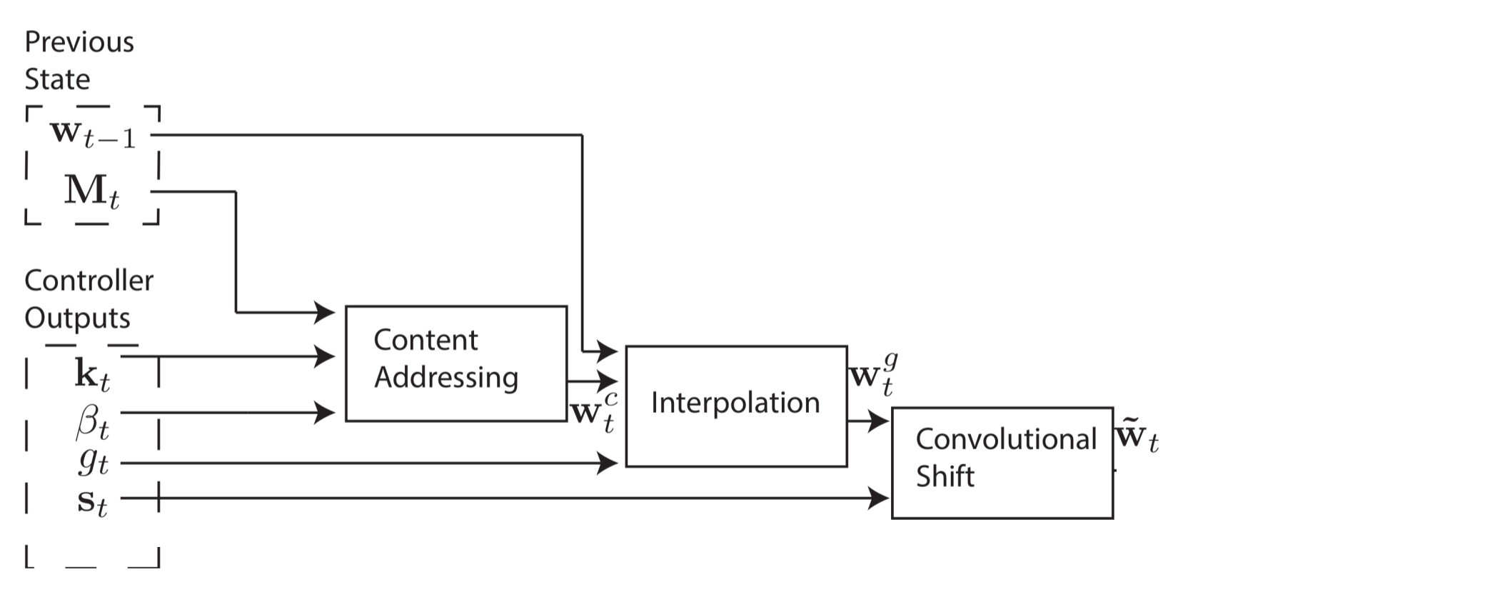
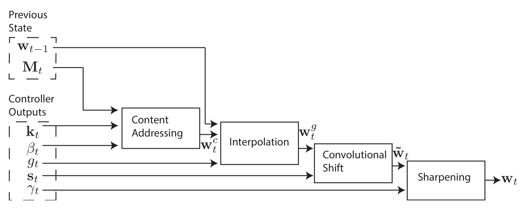
The fourth and final stage, refinement (sharpening), is used to prevent blurring of the weight of the shift . This requires a scalar .
Now it's done! You can calculate the weight vector, which defines the addresses to read and write. Even better, the system is fully differentiable and therefore has end-to-end end-to-end learning.
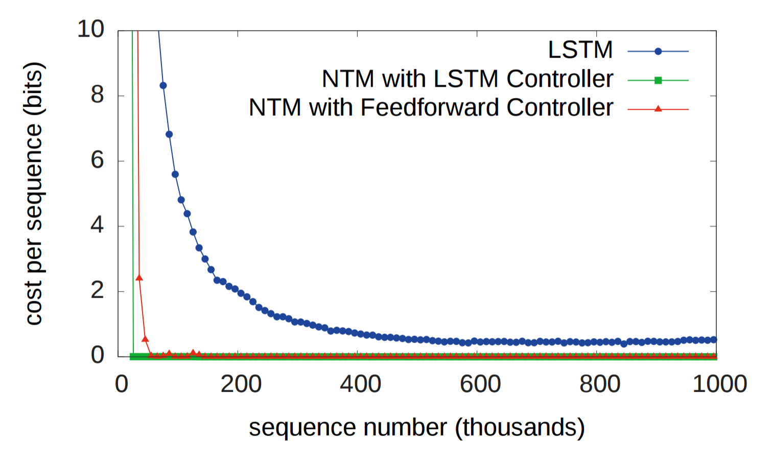
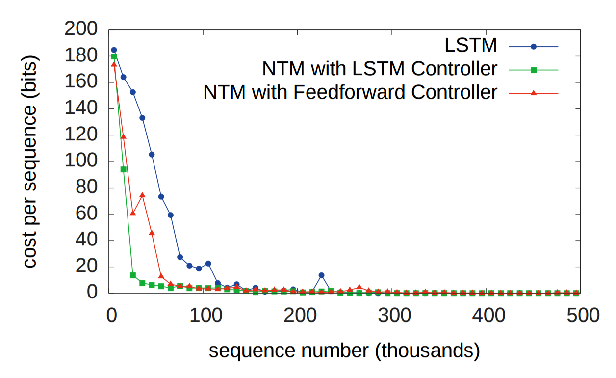
Historically, RNN suffered from the inability to permanently memorize information. The first experiment is designed to check whether the presence of an external memory system will improve the situation. In the experiment, the three systems were given a sequence of random eight-bit vectors, followed by the data separator flag, and then asked to repeat the sequence of input data. LSTM is compared with two NTMs, one of which uses an LSTM controller and the other uses a standard neural network (feedforward controller). In the graph below, the “cost function of each sequence” means the number of bits that the system incorrectly reproduced in the entire sequence. As you can see, both NTM architectures are far superior to LSTM.
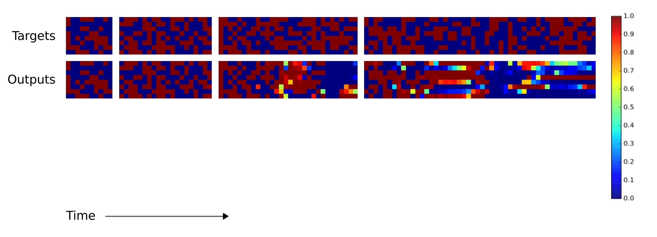
Obviously, both LSTM and NTM learned a certain rudimentary copying algorithm. The researchers graphically presented how NTM reads and writes (shown below). The white color corresponds to weight 1, and black to weight 0. The illustration clearly shows that the weights for the memory cells were clearly focused.

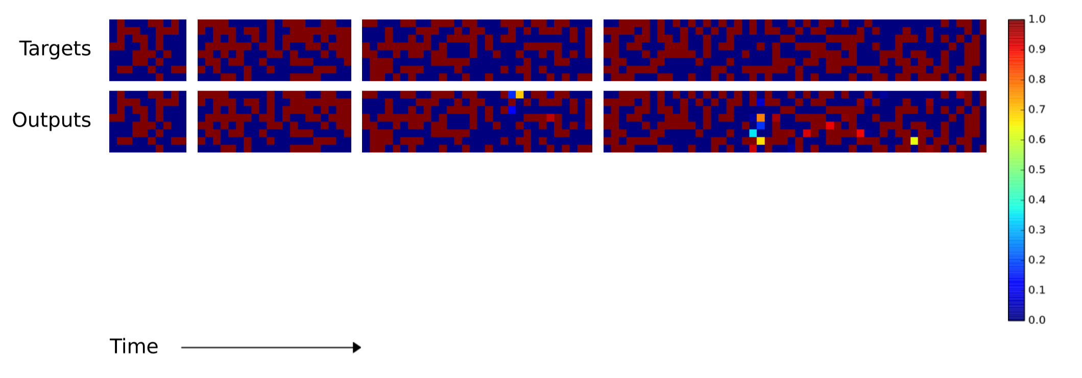
Next, the researchers wanted to know how well the LSTM and NTM algorithms can scale for longer sequences than all the input data they were trained on. Learning took place on sequences from 1 to 20 random vectors, so LSTM and NTM were compared on sequences of 10, 20, 30, 50 and 120 vectors. The following two illustrations need some explanation. There are eight blocks. The four upper blocks correspond to sequences 10, 20, 30, and 50. In each block, a column of eight red and blue squares is used to visualize the values of 1 and 0. The bright colored squares correspond to values between 0.0 and 1.0.
LSTM copy performance on sequences of length 10, 20, 30, 40
NTM copy performance on sequences of length 10, 20, 30, 40
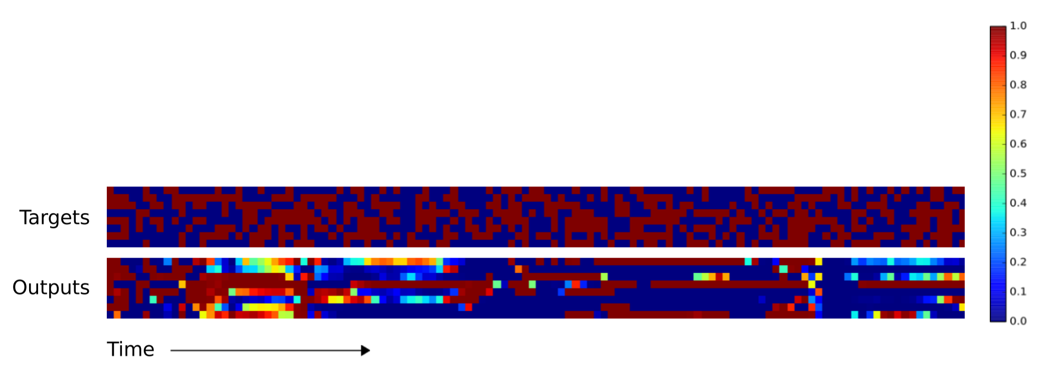
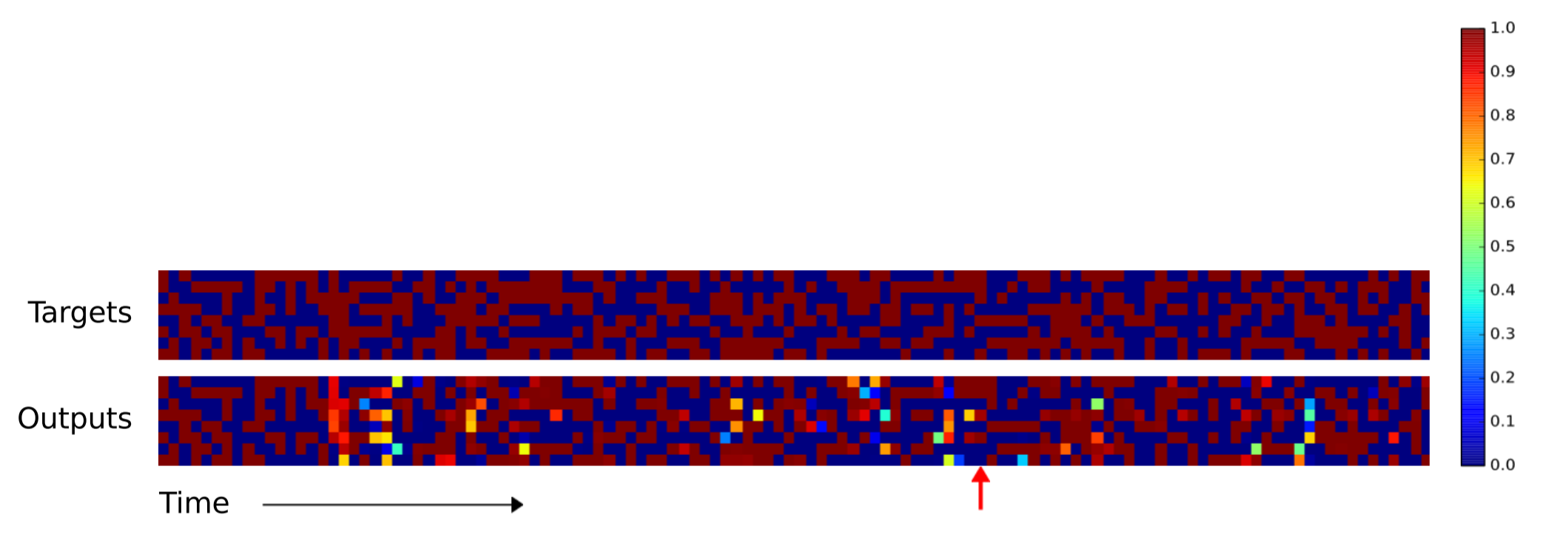
As you can see, NTM produces far fewer errors on long sequences. I could not find in scientific work exactly which NTM (RNN controller or proactive controller) was used when generating this image at the top. The difference between NTM and LSTM becomes even more pronounced as the sequence increases to 120 vectors, as shown below.
LSTM copy performance on 120 length sequences
NTM copy performance on 120-length sequences
The second experiment was to determine if NTM could learn the nested function (in this case, the nested loop). In addition to the sequence, a scalar value corresponding to the number of times NTM should output the copied input sequence was also transmitted to NTM. Both NTMs are expected to outperform LSTM.
As before, LSTM found it difficult to generalize the copy repetition algorithm, but NTM did not.

The third experiment was to determine if NTM was able to learn indirect handling, that is, when one data element points to another. The authors submitted a list of elements as input, and then requested one element from the list, waiting for the next element to be returned from the list. The authors note that the superiority of NTM with a preemptive controller over NTM with an LSTM controller indicates that NTM memory is a better data storage system than the internal state of LSTM.
Again, NTM surpassed LSTM when summarizing a large number of items in the list.
The fourth task was designed to determine whether NTM can learn a posteriori predictable distributions . The researchers created N-grams (sequences of N elements), which, when retrieving previous elements of a sequence, compute a certain probability distribution for the next element of the sequence. In this case, the researchers used binary 6-grams. The optimal solution for the agent's ability to predict the next bit will be the solution in an analytical form, and both NTM have exceeded the LSTM, approaching the optimal estimate.

The fifth and final experiment tested whether NTM could learn to sort the data. Twenty binary vectors were assigned scalar "priority ratings" evenly selected from the range [-1, 1], and the task of each system was to return the 16 vectors with the highest priority from the input data. After examining the write and read operations in the NTM memory, the scientists found that NTM roughly estimates the order in which order the vectors should be stored using priorities. Then, to output 16 vectors with the highest priority, the memory cells are read sequentially. This is evident in the sequence of operations, memorize and read from memory.
And once again, NTM surpassed LSTM.
I would be grateful for any feedback. If I made a mistake somewhere or if you have a suggestion, write to me or comment on Reddit and HackerNews . In the near future, I'm going to create a mailing list (thanks, Ben) and integrate RSS (thanks, Yuri).
Initially, I was not going to talk about this article, but I could not understand another interesting article I was going to talk about. It was about the NTM modification, so I decided to make sure I fully understand NTM before moving on. After verifying this, I had the feeling that that second article was not very suitable for explanation, but the original work on NTM was very well written, and I strongly recommend it to be read.
Motivation
During the first thirty years of artificial intelligence research, neural networks were considered mostly unpromising. From the 1950s to the late 1980s, the symbolic approach dominated AI. He assumed that the work of information processing systems like the human brain can be understood through manipulations with the symbols, structures, and rules of processing these symbols and structures. Only in 1986 appeared a serious alternative to symbolic AI; its authors used the term "parallel distributed processing" (Parallel Distributed Processing), but today the term " connectionism " is more often used. You might not have heard of such an approach, but you probably heard about one of the most famous connection modeling modeling techniques - artificial neural networks.
Critics have put forward two arguments against the fact that neural networks will help us better understand intelligence. Firstly, neural networks with a fixed size of input data, apparently, are not able to solve problems with input data of variable size. Secondly, neural networks seem to be unable to bind values to a specific location in data structures. The ability to write and read from memory is critical in both information processing systems that are available for study: in the brain and computers. In that case, what can be answered to these two arguments?
')
The first argument was refuted with the creation of recurrent neural networks (RNN). They can process variable-size input without needing to modify or add a time component to the processing procedure — when translating a sentence or recognizing handwritten text, RNN repeatedly receives input data of a fixed size as many times as required. In his scientific article, Graves et al. Tries to refute the second argument, giving the neural network access to external memory and the ability to learn how to use it. They called their system the Neural Turing Machine (NTM) .
Prerequisites
For specialists in computer theory, the need for a memory system is obvious. Computers have tremendously improved over the past half century, but they still consist of three components: memory, control logic, and arithmetic / logic operations. There are also biological evidence points to the benefits of a memory system for quickly storing and retrieving information. Such a memory system is called working memory , and the article on NTM refers to several earlier works that studied working memory from the point of view of computational neuroscience.
Intuition
The NTM schematic diagram includes a neural network called a controller , a 2D matrix (memory bank), and a memory matrix or ordinary memory . At each time step, the neural network receives some data from the outside world and sends some output to the outside world. However, the neural network also has the ability to read information from individual memory cells and the ability to write to individual memory cells. Graves et al. Drew inspiration from the traditional Turing machine and used the term “head” to describe memory cell operations. In the diagram below, the dashed line restricts parts of the architecture that are “inside” the system in relation to the outside world.
But there is a catch. Suppose we index the memory by specifying a row and column, as in a regular matrix. We would like to train our neural network using the error back-propagation method and our favorite optimization method (for example, the stochastic gradient method), but how to get a certain index gradient? Will not work. Instead, the controller performs read and write operations as part of “fuzzy” operations that interact with all the elements in memory to one degree or another. The controller will calculate the weights for the memory cells, which will allow it to determine the memory cells in a differentiated way. Next, I will explain how these weight vectors are generated, and then how they are used (it is easier to understand the system).
Maths
Reading
Take the memory matrix with rows and items in a row with time as . In order to read (and write), a certain attention mechanism is required, which determines where the head should read data from. The mechanism of attention will be normalized in length. (length- ) weight vector . We will talk about the individual elements of the weight vector as . By "rationing" authors imply the observance of the following two limitations:
The reading head will return the normalized length (length- ) vector which is a linear combination of strings of memory scaled by weight vector:
Record
Writing is a bit more complicated than reading because it involves two separate steps: erasing, then adding. To erase old data, the recording head needs a new vector, this is length- erase vector in addition to our length- normalized weight vector . The erase vector is used in conjunction with a weight vector to determine which elements in the line should be removed, left unchanged, or something in between. If the weight vector points to a line, and the erasing vector indicates an erase element, then the element in this line will be erased.
After conversion at the recording head uses length- adding vector to complete the write operation.
Addressing
Creating such weight vectors to determine where to read and write data is not easy, I would present this process in four stages. At each stage, an intermediate weight vector is generated, which is passed to the next stage. The goal of the first stage is to generate a weight vector based on how close each line in memory is to length. vector released by the controller. We will call this intermediate weight vector weight vector content. Other parameter I'll explain now.
The weight vector of the content allows the controller to select values that are similar to already known values, which is called content addressing. For each head, the controller produces a key vector. which is compared with each line using a measure of similarity. In this paper, the authors use the cosine measure of similarity, which is defined as follows:
Positive scalar parameter Which is called key strength is used to determine how concentrated the weight vector of the content should be. For small values of beta, the weight vector will be blurred, and for large values of beta, the weight vector will be concentrated on the most similar line in memory. For visualization, if the key and the memory matrix produce a similarity vector
[0.1, 0.5, 0.25, 0.1, 0.05] , this is how the weight vector of the content changes depending on the beta.Weight vector content can be calculated as follows:
However, in some cases we may want to read from specific memory cells, rather than read specific values in memory. For example, the authors show the function . In this case, we do not care about the specific values of x and y, only that they are constantly read from the same cells in memory. This is called cell addressing, and for its implementation we need three more steps. In the second stage, the scalar parameter which is called the interpolation gate, mixes the weight vector of the content with the weight vector of the previous time step for the production of valve weight vector . This allows the system to understand when to use (or ignore) content addressing.
We would like the controller to shift the focus to other lines. Suppose that one of the system parameters is limited to the range of allowable offsets. For example, the head's attention may shift forward one line (+1), remain unchanged (0), or move backward (-1) a line. Perform shifts by module so that moving forward from the bottom row of memory moves the head's attention to the top line, just as moving backward from the top line moves the head's attention to the bottom line. After interpolation, each head produces a normalized shift weighting. and the following convolutional movement occurs to calculate the weight of the shift .
The fourth and final stage, refinement (sharpening), is used to prevent blurring of the weight of the shift . This requires a scalar .
Now it's done! You can calculate the weight vector, which defines the addresses to read and write. Even better, the system is fully differentiable and therefore has end-to-end end-to-end learning.
Experiments and Results
Copying
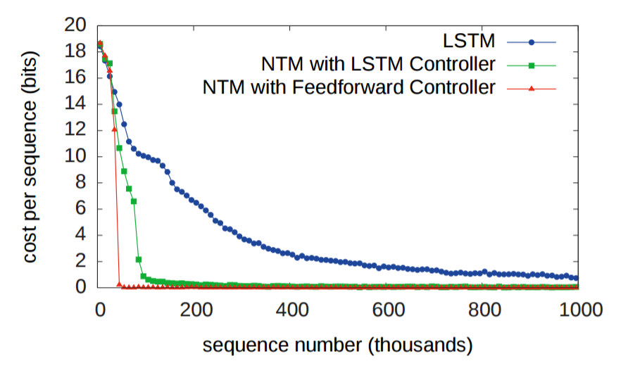
Historically, RNN suffered from the inability to permanently memorize information. The first experiment is designed to check whether the presence of an external memory system will improve the situation. In the experiment, the three systems were given a sequence of random eight-bit vectors, followed by the data separator flag, and then asked to repeat the sequence of input data. LSTM is compared with two NTMs, one of which uses an LSTM controller and the other uses a standard neural network (feedforward controller). In the graph below, the “cost function of each sequence” means the number of bits that the system incorrectly reproduced in the entire sequence. As you can see, both NTM architectures are far superior to LSTM.
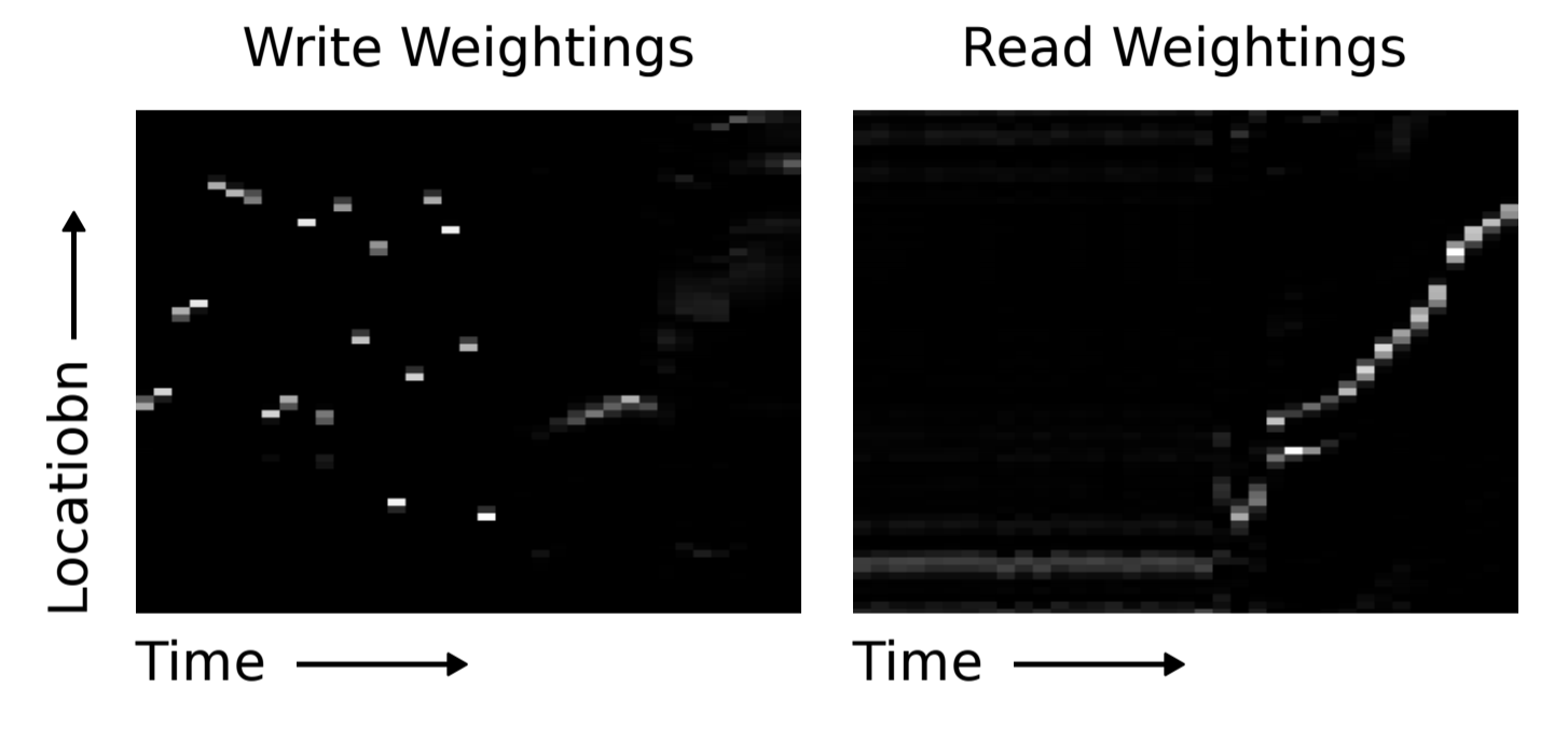
Obviously, both LSTM and NTM learned a certain rudimentary copying algorithm. The researchers graphically presented how NTM reads and writes (shown below). The white color corresponds to weight 1, and black to weight 0. The illustration clearly shows that the weights for the memory cells were clearly focused.
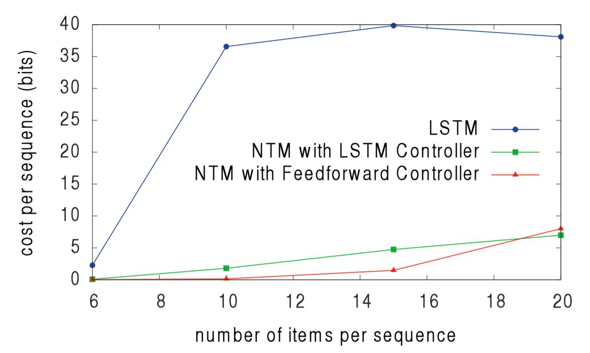
Next, the researchers wanted to know how well the LSTM and NTM algorithms can scale for longer sequences than all the input data they were trained on. Learning took place on sequences from 1 to 20 random vectors, so LSTM and NTM were compared on sequences of 10, 20, 30, 50 and 120 vectors. The following two illustrations need some explanation. There are eight blocks. The four upper blocks correspond to sequences 10, 20, 30, and 50. In each block, a column of eight red and blue squares is used to visualize the values of 1 and 0. The bright colored squares correspond to values between 0.0 and 1.0.
LSTM copy performance on sequences of length 10, 20, 30, 40
NTM copy performance on sequences of length 10, 20, 30, 40
As you can see, NTM produces far fewer errors on long sequences. I could not find in scientific work exactly which NTM (RNN controller or proactive controller) was used when generating this image at the top. The difference between NTM and LSTM becomes even more pronounced as the sequence increases to 120 vectors, as shown below.
LSTM copy performance on 120 length sequences
NTM copy performance on 120-length sequences
Re-copy
The second experiment was to determine if NTM could learn the nested function (in this case, the nested loop). In addition to the sequence, a scalar value corresponding to the number of times NTM should output the copied input sequence was also transmitted to NTM. Both NTMs are expected to outperform LSTM.
As before, LSTM found it difficult to generalize the copy repetition algorithm, but NTM did not.
Associative data recovery
The third experiment was to determine if NTM was able to learn indirect handling, that is, when one data element points to another. The authors submitted a list of elements as input, and then requested one element from the list, waiting for the next element to be returned from the list. The authors note that the superiority of NTM with a preemptive controller over NTM with an LSTM controller indicates that NTM memory is a better data storage system than the internal state of LSTM.
Again, NTM surpassed LSTM when summarizing a large number of items in the list.
Dynamic N-grams
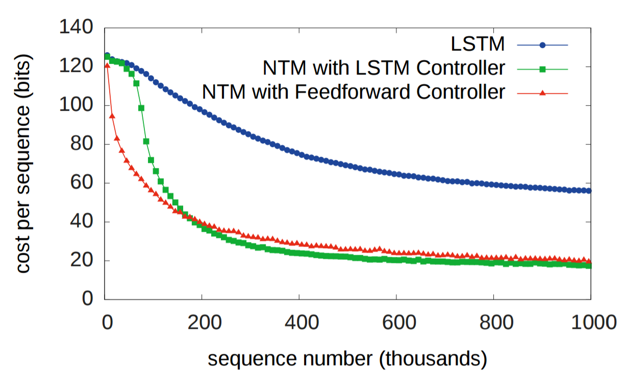
The fourth task was designed to determine whether NTM can learn a posteriori predictable distributions . The researchers created N-grams (sequences of N elements), which, when retrieving previous elements of a sequence, compute a certain probability distribution for the next element of the sequence. In this case, the researchers used binary 6-grams. The optimal solution for the agent's ability to predict the next bit will be the solution in an analytical form, and both NTM have exceeded the LSTM, approaching the optimal estimate.
Priority sorting
The fifth and final experiment tested whether NTM could learn to sort the data. Twenty binary vectors were assigned scalar "priority ratings" evenly selected from the range [-1, 1], and the task of each system was to return the 16 vectors with the highest priority from the input data. After examining the write and read operations in the NTM memory, the scientists found that NTM roughly estimates the order in which order the vectors should be stored using priorities. Then, to output 16 vectors with the highest priority, the memory cells are read sequentially. This is evident in the sequence of operations, memorize and read from memory.
And once again, NTM surpassed LSTM.
Summary
- Neurobiological models of working brain memory and digital computer architecture suggest that the functionality of the system may depend on the availability of external memory.
- Neural networks, supplemented by external memory, offer a possible answer to a key critical argument in the direction of connectivism, that neural networks are not able to bind values to a specific location in data structures (linking variables).
- Blurry read and write operations are differentiable. This is critical for the controller to learn how to use memory.
- The results of the five tests showed that NTM can outperform LSTM and learn more generalized algorithms than LSTM.
Notes
I would be grateful for any feedback. If I made a mistake somewhere or if you have a suggestion, write to me or comment on Reddit and HackerNews . In the near future, I'm going to create a mailing list (thanks, Ben) and integrate RSS (thanks, Yuri).
Source: https://habr.com/ru/post/327614/
All Articles