Open machine learning course. Theme 10. Gradient boosting
Hello! It is time to replenish our algorithmic arsenal with you.
Today we will thoroughly analyze one of the most popular and applied in practice machine learning algorithms - gradient boosting. It’s about where the roots grow from the busting and what’s really going on under the hood of the algorithm - in our colorful journey into the world of busting under the cat.
UPD: now the course is in English under the brand mlcourse.ai with articles on Medium, and materials on Kaggle ( Dataset ) and on GitHub .
Video recording of the lecture based on this article in the second run of the open course (September-November 2017).
- Primary data analysis with Pandas
- Visual data analysis with Python
- Classification, decision trees and the method of nearest neighbors
- Linear classification and regression models
- Compositions: bagging, random forest. Validation and training curves
- Construction and selection of signs
- Teaching without a teacher: PCA, clustering
- We study on gigabytes with Vowpal Wabbit
- Time Series Analysis with Python
- Gradient boosting
Plan for this article:
- Introduction and history of boosting
- GBM algorithm
- Loss functions
- The result of the theory of GBM
- Homework
- useful links
1. Introduction and history of the appearance of boosting
Most people involved in data analysis have heard about boosting at least once. This algorithm is included in the daily "gentleman's set" of models that are worth trying in the next task. Xgboost is often associated with a standard recipe for winning in ML competitions , giving rise to a meme about “pack xgboost”. And also boosting is an important part of most search engines , sometimes speaking also as their business card . Let's look at the overall development as a boosting appeared and developed.
The history of the appearance of boosting
It all started with the question of whether it is possible to get one strong out of a large number of relatively weak and simple models. By weak models, we mean not just small and simple models like decision trees as opposed to more “strong” models, such as neural networks. In our case, weak models are arbitrary machine learning algorithms, the accuracy of which can only be slightly higher than random guessing.
The affirmative mathematical answer to this question was found rather quickly , which in itself was an important theoretical result (a rarity in ML). However, it took several years before the advent of working algorithms and Adaboost. Their general approach was to greedily build a linear combination of simple models (basic algorithms) by reweighing the input data. Each subsequent model (as a rule, a decision tree) was constructed in such a way as to give more weight and preference to previously incorrectly predicted observations.
In an amicable way, we should follow the example of most of the rest of the machine learning courses, and before the gradient boosting we carefully analyze its predecessor - Adaboost. However, we decided to go straight to the most interesting, because Adaboost eventually merged with GBM when it became clear that this was just its private variation.
The algorithm itself has a very visual visual interpretation of the intuition of observation weighing behind it. Consider a toy example of a classification problem in which we will try at each iteration of Adaboost to separate data from a tree of depth 1 (the so-called “stump”). In the first two iterations we will see the following image:
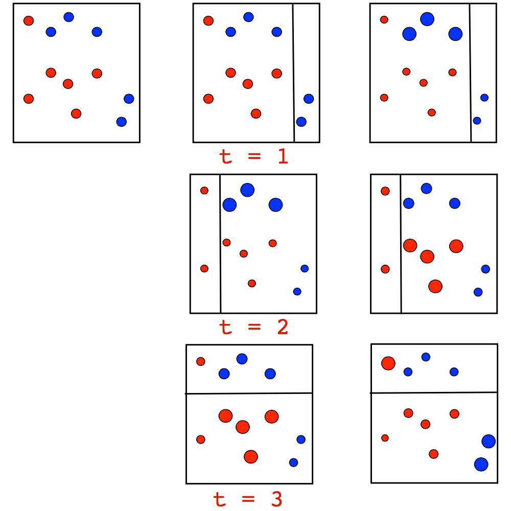
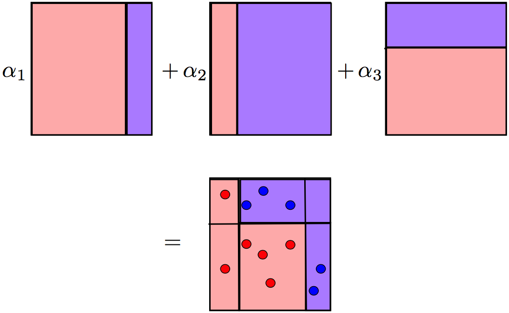
The size of the point corresponds to the weight it received for an erroneous prediction. And we see how, at each iteration, these weights grow - stumps cannot alone cope with such a task. However, when we make a weighted vote of previously constructed stumps, we will get the division we are looking for:
A more detailed example of the work of Adaboost, which shows a consistent increase in points over a series of iterations, especially at the border between the classes:
Adaboost worked well, but due to the fact that there were few substantiations of the algorithm with its add-ons, a full range of speculations arose around them: someone thought it was an over-algorithm and a magic bullet, someone was skeptical and inapplicable approach with hard re-fitting (overfitting). This was particularly true of the applicability of data with powerful outliers, to which Adaboost was unstable. Fortunately, when the professorship of the Stanford department of statistics took over the business, which already brought the world Lasso, Elastic Net and Random Forest, in 1999 Jerome Friedman introduced a generalization of the developments of the algorithms of boosting - gradient boosting, also known as Gradient Boosting (Machine), also GBM. With this work, Friedman immediately set the statistical base for creating many algorithms, providing a general approach of boosting as optimization in the functional space.
In general, the team at Stanford Statistics Department is involved in CART, bootstrap, and many other things, having pre-entered their names in future statistics textbooks. By and large, a significant part of our everyday toolkit appeared exactly there, and who knows what else will appear. Or it has already appeared, but has not yet found enough distribution (as, for example, glinternet ).
There are not many videos with Friedman himself. However, there is a very interesting interview with him about the creation of CART, and in general about how to solve statistical problems (which we would attribute to data analysis and data science) 40+ years ago:
From the series of a cognitive history of data analysis, there is also a lecture from Hastie with a retrospective of data analysis from one of the participants in creating our daily methods with you:
In fact, there was a transition from engineering-algorithmic research in the construction of algorithms (so characteristic in ML) to a full-fledged methodology, such as building and studying such algorithms. From the point of view of the mathematical stuffing, at first glance, not so much has changed: we are also adding (boosting) weak algorithms, building up our ensemble with gradual improvements in those sections of data where the previous models have not “finalized”. But when building the following simple model, it is built not simply on re-weighted observations, but in a way that best approximates the overall gradient of the objective function. At the conceptual level, it gave a lot of room for imagination and extensions.
History of the formation of GBM
Gradient boosting did not take its place in the “gentleman's set” immediately - it took more than 10 years from the moment it appeared. First, the base GBM has many extensions for different statistical tasks: GLMboost and GAMboost as an enhancement of existing GAM models, CoxBoost for survival curves, RankBoost and LambdaMART for ranking. Secondly, there are many implementations of the same GBM under different names and different platforms: Stochastic GBM, GBDT (Gradient Boosted Decision Trees), GBRT (Gradient Boosted Regression Trees), MART (Multiple Additive Regression Trees), GBM as Generalized Boosting Machines and other In addition, the machine learner communities were rather fragmented and engaged in everything in a row, because of this, tracking the success of the boosting is quite difficult.
At the same time, boosting began to be actively used in ranking tasks for search engines. This task was written from the point of view of the loss function, which penalizes errors in the order of issue, so that it became convenient to simply insert it into GBM. One of the first to introduce a boosting into the ranking of AltaVista, and soon followed by Yahoo, Yandex, Bing and others. Moreover, speaking of implementation, it was about the fact that boosting for years to come became the main algorithm within the operating engines, and not another interchangeable research hack living within a couple of scientific articles.
 The main role in promoting the boosting was played by ML competitions, especially kaggle. Researchers have long lacked a common platform where there would be enough participants and tasks to compete in an open struggle for the state of the art with their algorithms and approaches. The gloomy German geniuses who grew up in their garage next miracle algorithm could not all be written off as private data, and real breakthrough libraries on the contrary received an excellent platform for development. This is exactly what happened with the boosting, which took root on kaggle almost immediately (GBM was found in an interview with the winners from 2011), and xgboost as a library quickly gained popularity soon after its appearance. At the same time, xgboost is not some kind of new unique algorithm, but simply an extremely effective implementation of classical GBM with some additional heuristics.
And here we are, in 2017, we use an algorithm that went very typical for ML from mathematical problem and algorithmic handicrafts through the emergence of normal algorithms and normal methodology to successful practical applications and mass use years after its appearance.
2. GBM algorithm
Setting ML task
We will solve the task of restoring a function in the general context of training with a teacher. We will have a set of pairs of signs l a r g e x and target variables l a r g e y , \ large \ left \ {(x_i, y_i) \ right \} _ {i = 1, \ ldots, n}\ large \ left \ {(x_i, y_i) \ right \} _ {i = 1, \ ldots, n} on which we will restore the dependence of the form largey=f(x) . We will restore the approximation large hatf(x) , and to understand which approximation is better, we will also have a loss function largeL(y,f) which we will minimize:
largey approx hatf(x), large hatf(x)= undersetf(x) arg min L(y,f(x))
So far, we have not made any assumptions about the type of dependence largef(x) nor about our approximation model large hatf(x) nor about the distribution of the target variable largey . Is that a function largeL(y,f) should be differentiable. Since the problem must be solved not on all the data in the world, but only on those at our disposal, we will rewrite everything in terms of mathematical expectations. Namely, we will search for our approximations. large hatf(x) so that, on average, to minimize the loss function on the data that is:
large hatf(x)= undersetf(x) arg min mathbbEx,y[L(y,f(x))]
Unfortunately, the functions largef(x) there is not just a lot in the world - their very functional space is infinite-dimensional. Therefore, in order to at least somehow solve the problem, in machine learning they usually limit the search space to some specific parameterized family of functions. largef(x, theta), theta in mathbbRd . This greatly simplifies the task, since it boils down to the already completely solvable optimization of parameter values:
large hatf(x)=f(x, hat theta), large hat theta= underset theta arg min mathbbEx,y[L(y,f(x, theta))]
Analytical solutions for optimal parameters large hat theta in one line there are rarely enough, so the parameters are usually approximated iteratively. First we need to write out the empirical loss function largeL theta( hat theta) showing how well we rated them based on the data we have. We will also write out our approximation. large hat theta behind largeM iterations as a sum (and for clarity, and to start getting used to boosting):
large hat theta= sumMi=1 hat thetai, largeL theta( hat theta)= sumNi=1L(yi,f(xi, hat theta))
Things are going to be small - it remains only to take a suitable iterative algorithm, which we will minimize largeL theta( hat theta) . The simplest and most commonly used option is gradient descent. For him, you need to write a gradient large nablaL theta( hat theta) and add our iterative evaluations large hat thetai along it (with a minus sign - we want to reduce the error, not increase). And that's all, you just need to somehow initialize our first approximation. large hat theta0 and choose how many iterations largeM we will continue this procedure. In our memory-ineffective storage of approximations large hat theta The naive algorithm will look like this:
- Initialize initial parameter approximation large hat theta= hat theta0
- For each iteration larget=1, dots,M to repeat:
- Calculate the loss function gradient large nablaL theta( hat theta) at the current approximation large hat theta
large nablaL theta( hat theta)= left[ frac partialL(y,f(x, theta)) partial theta right] theta= hat theta - Set current iterative approximation large hat thetat based on counted gradient
large hat thetat leftarrow− nablaL theta( hat theta) - Update parameter approximation large hat theta :
large hat theta leftarrow hat theta+ hat thetat= sumti=0 hat thetai
- Calculate the loss function gradient large nablaL theta( hat theta) at the current approximation large hat theta
- Save final approximation large hat theta
large hat theta= sumMi=0 hat thetai - Use the function found large hatf(x)=f(x, hat theta) as intended
Functional Gradient Descent
Expand consciousness: imagine for a second that we can carry out optimization in the functional space and iteratively search for approximations large hatf(x) in the form of the functions themselves. We write out our approximation as the sum of incremental improvements, each of which is a function. For convenience, we will immediately assume this amount, starting with the initial approximation large hatf0(x) :
large hatf(x)= sumMi=0 hatfi(x)
Magic has not happened yet, we just decided that we would look for our approach large hatf(x) not as one large model with a bunch of parameters (like, for example, a neural network), but as a sum of functions, pretending that in this way we move in a functional space.
To solve the problem, we still have to limit our search to some family of functions. large hatf(x)=h(x, theta) . But, first, the sum of the models can be more complicated than any model from this family (the sum of two trees-stumps of depth 1 is no longer close by one stump). Secondly, the overall task still occurs in the functional space. Immediately take into account, at each step for the functions we need to select the optimal coefficient large rho in mathbbR . For step larget The task is as follows:
large hatf(x)= sumt−1i=0 hatfi(x), large( rhot, thetat)= underset rho, theta arg min mathbbEx,y[L(y, hatf(x)+ rho cdoth(x, theta))], large hatft(x)= rhot cdoth(x, thetat)
And now is the time of magic. We wrote out all our tasks in a general way, as if we could just take and train all kinds of models largeh(x, theta) regarding any loss functions largeL(y,f(x, theta)) . In practice, this is extremely difficult, so a simple way to reduce the problem to something solvable was invented.
Knowing the expression of the loss function gradient, we can calculate its values on our data. So let's train models so that our predictions are most correlated with this gradient (with a minus sign). That is, we will solve the OLS-regression problem, trying to correct the predictions for these residues. And for classification, and for regression, and for ranking under the hood, we will all the time minimize the squared difference between the pseudo-residues larger and our predictions. For step larget The final task is as follows:
large hatf(x)= sumt−1i=0 hatfi(x), largerit=− left[ frac partialL(yi,f(xi)) partialf(xi) right]f(x)= hatf(x), quad mboxfori=1, ldots,n, large thetat= underset theta arg min sumni=1(rit−h(xi, theta))2, large rhot= underset rho arg min sumni=1L(yi, hatf(xi)+ rho cdoth(xi, thetat))

Classic GBM Friedman Algorithm
Now we have everything we need to finally write out the GBM algorithm proposed by Jerome Friedman in 1999. We still solve the general problem of learning with the teacher. At the input of the algorithm you need to collect several components:
- data set \ large \ left \ {(x_i, y_i) \ right \} _ {i = 1, \ ldots, n}\ large \ left \ {(x_i, y_i) \ right \} _ {i = 1, \ ldots, n} ;
- number of iterations largeM ;
- loss function selection largeL(y,f) with drawn gradient;
- selection of a family of functions for basic algorithms largeh(x, theta) , with the procedure of their training;
- additional hyperparameters largeh(x, theta) for example, the depth of a tree in decision trees;
The only moment left unattended is the initial approach. largef0(x) . For simplicity, just a constant value is used as initialization. large gamma . His, as well as the optimal ratio large rho find a binary search, or another line search algorithm relative to the original loss function (and not the gradient). So, GBM algorithm:
- Initialize GBM constant value large hatf(x)= hatf0, hatf0= gamma, gamma in mathbbR
large hatf0= underset gamma arg min sumni=1L(yi, gamma) - For each iteration larget=1, dots,M to repeat:
- Count pseudo-residues largert
largerit=− left[ frac partialL(yi,f(xi)) partialf(xi) right]f(x)= hatf(x), quad mboxfori=1, ldots,n - Build a new basic algorithm largeht(x) as regression on pseudo-residues \ large \ left \ {(x_i, r_ {it}) \ right \} _ {i = 1, \ ldots, n}\ large \ left \ {(x_i, r_ {it}) \ right \} _ {i = 1, \ ldots, n}
- Find the optimal ratio large rhot at largeht(x) relative to the original loss function
large rhot= underset rho arg min sumni=1L(yi, hatf(xi)+ rho cdoth(xi, theta)) - Save large hatft(x)= rhot cdotht(x)
- Update current approximation large hatf(x)
large hatf(x) leftarrow hatf(x)+ hatft(x)= sumti=0 hatfi(x)
- Count pseudo-residues largert
- Build the resulting GBM model large hatf(x)
large hatf(x)= sumMi=0 hatfi(x) - To conquer the kaggle and the world with a trained model (you will understand the predictions there yourself)
GBM step by step example
Let's try on a toy example to figure out how GBM works. We will use it to restore the noisy function. largey=cos(x)+ epsilon, epsilon sim mathcalN(0, frac15),x in[−5.5] .
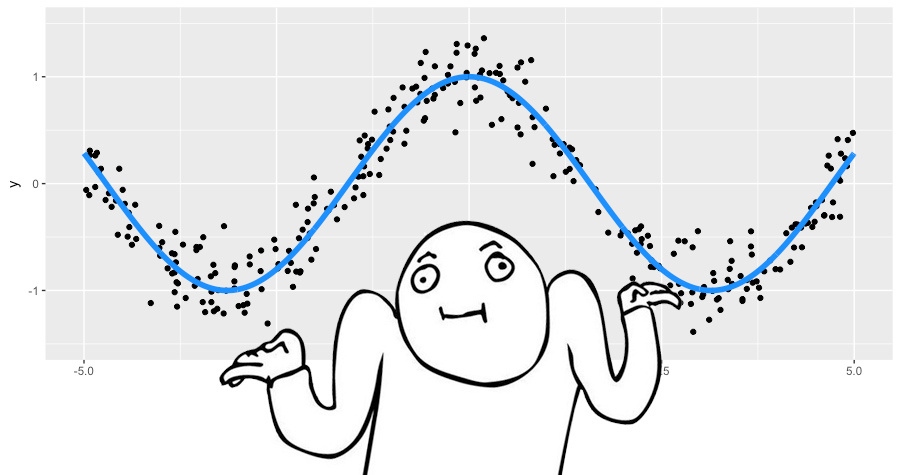
This is a regression problem for a real target variable, so we use the mean square loss function. We will generate 300 pairs of observations, and we will approximate by decision trees of depth 2. Let's put together everything we need to use GBM:
- Toy data \ large \ left \ {(x_i, y_i) \ right \} _ {i = 1, \ ldots, 300}\ large \ left \ {(x_i, y_i) \ right \} _ {i = 1, \ ldots, 300} ✓
- Number of iterations largeM=3 ✓;
- RMS loss function largeL(y,f)=(y−f)2 ✓
Gradient largeL(y,f)=L2 loss is just a remnant larger=(y−f) ✓; - Decision trees as basic algorithms largeh(x) ✓;
- Hyperparameters of decision trees: the depth of the trees is 2 ✓;
RMS error is simple and initialized large gamma and with coefficients large rhot . Namely, we initialize GBM we will average large gamma= frac1n cdot sumni=1yi , and all large rhot equal to 1.
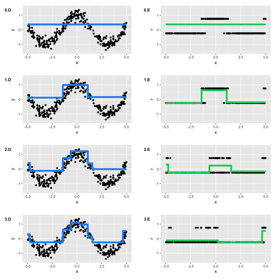
Run GBM and draw two types of graphs: current approximation large hatf(x) (blue graph), as well as every tree built large hatft(x)on their pseudo-residues (green graph). The number of the graph corresponds to the number of the iteration:
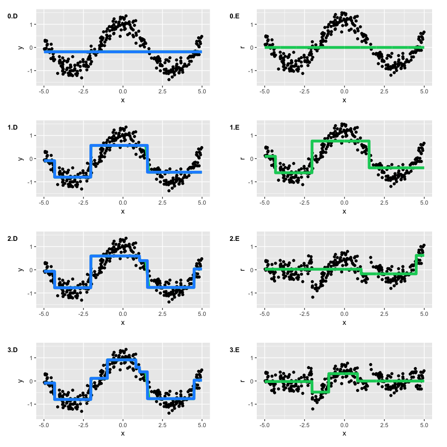
Note that by the second iteration, our trees repeated the basic form of the function. However, at the first iteration, we see that the algorithm built only the "left branch" of the function (x∈[−5,−4] ).It turned out to be banal because our trees did not have enough depth to build a symmetrical branch right away, and the error on the left branch was greater. So, the right branch "sprouted" only on the second iteration.
: - , GBM . , , GBM , . , GBM , Brilliantly wrong :
3.
, , , , ? , y L(y,f) . , , .
, — . : y∈R y∈{−1,1} . , , , .
y∈R . , , (y|x) . :
- L(y,f)=(y−f)2 , L2 loss, Gaussian loss. , . () — .
- L(y,f)=|y−f| , L1 loss, Laplacian loss. , , , . , , , , , .
- , Lq loss, Quantile loss. , , L1 , 75%-, α=0.75 . , , .
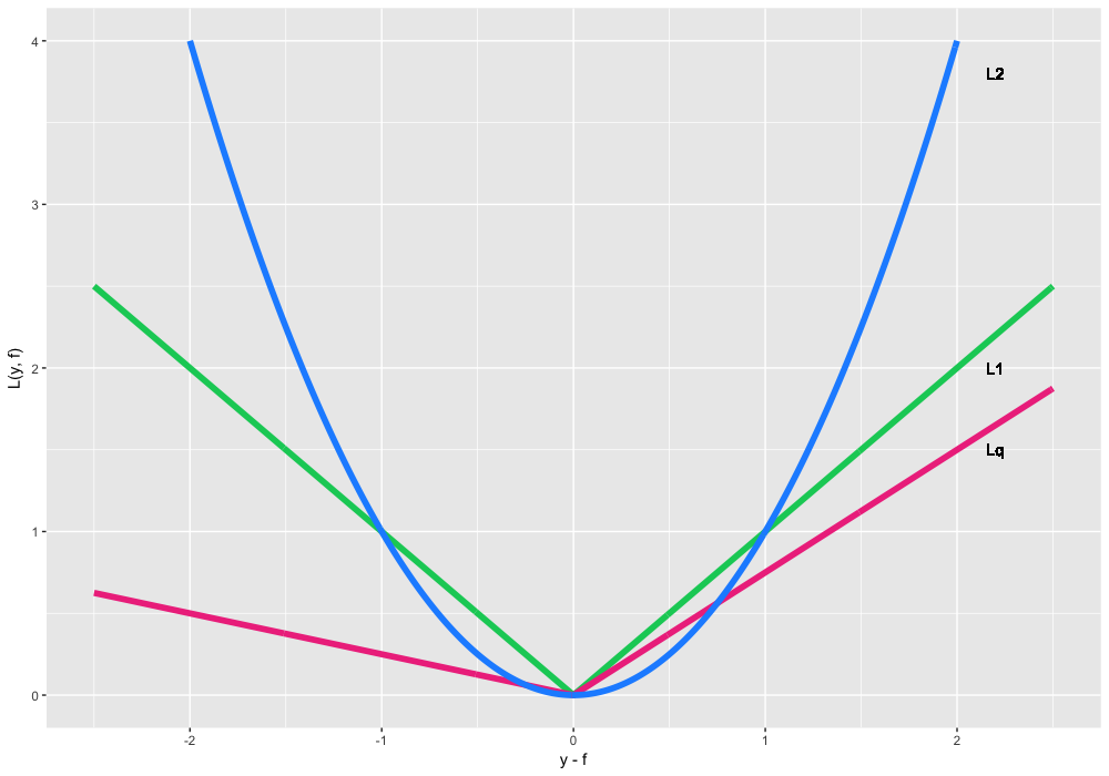
Lq , 75%- . :
- {(xi,yi)}i=1,…,300 ✓
- M=3 ✓;
- ✓;
- Gradient L0.75(y,f) — , α=0.75 . -, :
ri=−[∂L(yi,f(xi))∂f(xi)]f(x)=ˆf(x)=
=αI(yi>ˆf(xi))−(1−α)I(yi≤ˆf(xi)),for i=1,…,300 ✓; - h(x) ✓;
- : 2 ✓;
We have an obvious initial approximation - just take the quantile we need y . However, about optimal ratios ρtwe don't know anything, so let's use the standard line search. Let's see what we got:
It's unusual to see that in fact we teach something very different from ordinary residues - at each iteration largeri accept only two possible values. However, the output of GBM is quite similar to our original function.
If you leave the algorithm to learn from this toy example, we get almost the same result as with the quadratic loss function, shifted by large approx$0.13 . But if we were looking for quantiles above 90%, computational difficulties might arise. Namely, if the ratio of the number of points above the desired quantile is too small (as unbalanced classes), the model will not be able to learn well. It is worth thinking about such nuances when solving atypical tasks.
For the regression problem, quite a lot of loss functions have been developed, including those with additional robustness properties. One such example is the loss function of Huber, aka Huber loss . The essence of the function is that on small deviations it works as largeL2 , and from a predetermined threshold, begins to work as largeL1 . This allows you to reduce the contribution of emissions and the following quadratically large errors on the general form of the function, while not focusing on minor inaccuracies and deviations.
You can see how this loss function works in the following toy example. Let's take the toy function data as a basis. largey= fracsin(x)x , to which a special noise was added: a mixture of the Gaussian distribution and the Bernoulli distribution, which acts as a one-way emission generator. The loss functions themselves are shown in graphs AD, and the corresponding GBMs in graphs FH (in graph E, the original function):
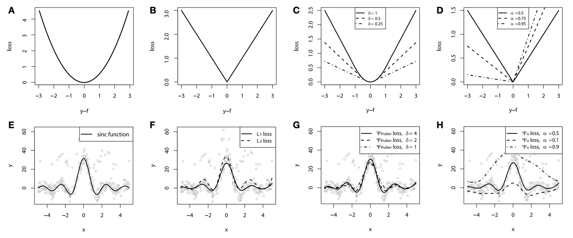
In this example, splines were used as basic algorithms for visual clarity. We have already said that you can not only plant trees?
According to the results of the example, due to the artificially created noise problem, the difference between largeL2 , largeL1 and Huber loss is quite noticeable. With proper selection of the parameter Huber loss, we even get the best approximation of the function among our options. And in this example, the difference in conditional quantiles is clearly visible (10%, 50% and 90% in our case).
Unfortunately, the Huber loss function is not implemented in all modern libraries (in h2o it is implemented, in xgboost not yet). The same applies to other interesting loss functions, including conditional quantiles, and such exotic things as conditional expects . But in general, it is quite useful to know that such options exist and can be used.
Loss classification functions
Now we will analyze the binary classification when \ large y \ in \ left \ {- 1, 1 \ right \} . We have already seen that even non-differentiable loss functions can be optimized using GBM. And in general, it would be possible, without thinking, to try to solve this case as another regression problem with some largeL2 loss, but it will not be very correct (although possible).
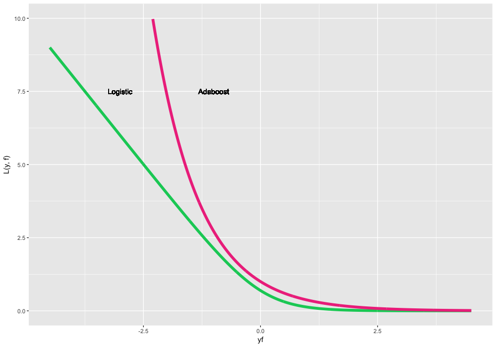
Due to the fundamentally different nature of the distribution of the target variable, we will predict and optimize not the class labels themselves, but their log-likelihood. To do this, we reformulate the loss functions over the multiplied predictions and true labels. largey cdotf (it’s not by chance that we chose labels of different signs). The most well-known variants of such classification loss functions:
- largeL(y,f)=log(1+exp(−2yf)) , it is Logistic loss, it is Bernoulli loss. An interesting property is that we penalize even correctly predicted class labels. No, this is not a bug. On the contrary, by optimizing this loss function, we can continue to “push” classes and improve the classifier even if all observations are correctly predicted. This is the most standard and frequently used loss function in a binary classification.
- largeL(y,f)=exp(−yf) it is Adaboost loss. It so happened that the classic Adaboost algorithm is equivalent to GBM with this loss function. Conceptually, this loss function is very similar to Logistic loss, but it has a tougher exponential penalty for classification errors and is used less frequently.
We will generate new toy data for the classification task. We take our noisy cosine as a basis, and we will use the function sign as the classes of the target variable. New data is as follows (jitter-noise added for clarity):
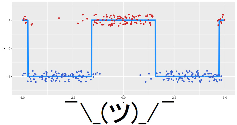
We will use Logistic loss to see what we are actually driving. As before, we put together what we will decide:
- Toy data \ large \ left \ {(x_i, y_i) \ right \} _ {i = 1, \ ldots, 300}, y_i \ in \ left \ {- 1, 1 \ right \} ✓
- Number of iterations largeM=3 ✓;
- As a loss function - Logistic loss, its gradient is considered as follows:
largeri= frac2 cdotyi1+exp(2 cdotyi cdot hatf(xi)), quad mboxfori=1, ldots,$30 ✓; - Decision trees as basic algorithms largeh(x) ✓;
- Hyperparameters of decision trees: the depth of the trees is 2 ✓;
This time, with the initialization of the algorithm, everything is a bit more complicated. First, our classes are unbalanced and divided in proportion of approximately 63% to 37%. Secondly, the analytical formula for initialization for our loss function is unknown. So we will look for large hatf0= gamma search:
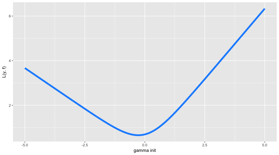
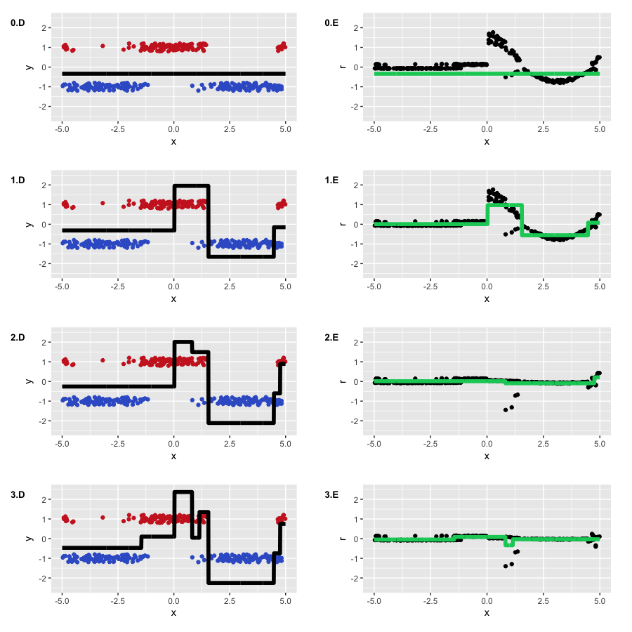
The optimal initial approximation was found at -0.273. One could guess that it will be negative (it is more profitable for us to predict all of the most popular class), but formulas of exact value, as we have said, no. And now let's finally launch GBM and see what actually happens under its hood:
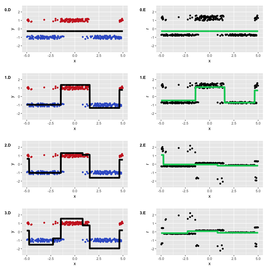
The algorithm worked successfully, restoring the separation of our classes. You can see how the "lower" areas are separated, in which the trees are more confident in the correct prediction of the negative class, and how two steps are formed where the classes were mixed. On the pseudo-remnants, it is clear that we have quite a few correctly classified observations, and a certain number of observations with large errors, which appeared due to noise in the data. Something looks like what GBM actually predicts in the classification problem (regression on pseudo-residuals of the logistic loss function).
Weights
Sometimes there is a situation when the task wants to come up with a more specific loss function. For example, in predicting financial series, we may want to give more weight to large movements of the time series, and in the task of predicting customer churn, it is better to predict churn from clients with high LTV (lifetime value, how much money the client will bring in the future).
The true path of a statistical warrior is to come up with his own loss function, write a derivative for it (and for more effective training, also the Hessian), and carefully check whether this function satisfies the required properties. However, there is a high probability of somewhere to be mistaken, to face computational difficulties, and, in general, to spend an inadmissibly long time on research.
Instead, a very simple tool was invented, which is rarely remembered in practice - weighing observations and setting weight functions. The simplest example of such a weighting is the assignment of weights for balancing classes. In general, if we know that some kind of subset of data, as in the input variables largex and in the target variable largey is more important for our model, we just give them more weight largew(x,y) . The main thing is to fulfill the general requirements of the rationality of the scales:
largewi in mathbbR, largewi geq0 quad mboxfori=1, ldots,n, large sumni=1wi>$
Weights can significantly reduce the time to adjust the loss function itself for the problem being solved, and also encourage experiments with the target properties of the models. How exactly to set these weights is exclusively our creative task. From the point of view of the GBM algorithm and optimization, we simply add scalar weights, closing our eyes to their nature:
largeLw(y,f)=w cdotL(y,f), largerit=−wi cdot left[ frac partialL(yi,f(xi)) partialf(xi) right]f(x)= hatf(x), quad mboxfori=1, ldots,n
It is clear that for arbitrary weights we do not know any beautiful statistical properties of our model. In general, tying the weights to the values largey , we can shoot our knee. For example, using weights proportional to large|y| at largeL1 loss function - not equivalent largeL2 loss, since the gradient will not take into account the values of the predictions themselves large hatf(x) .
We discuss all this in order to better understand our capabilities. Let's think up some very exotic example of scales on our toy data. We assign a strongly asymmetric weight function as follows:
$$ display $$ \ large \ begin {equation} w (x) = \ left \ {\ begin {array} {@ {} ll @ {}} 0.1, & \ text {if} \ x \ leq 0 \\ 0.1 + | cos (x) |, & \ text {if} \ x> 0 \ end {array} \ right. \ end {equation} $$ display $$
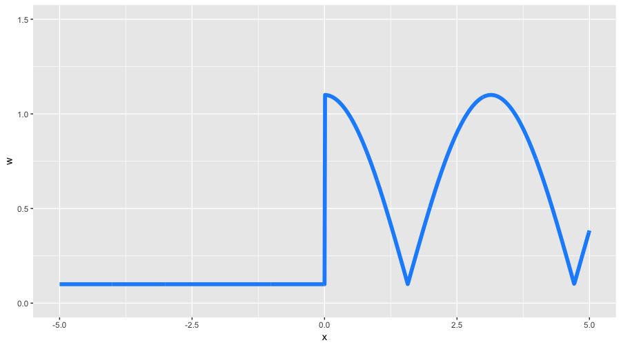
With these weights, we expect to see two properties: less detail on negative values. largex , and also the form of the function, to a greater degree similar to the original cosine. All other GBM settings we take from our previous classification example, including line search for optimal coefficients. Let's see what we got:
The result was what we expected. First, it can be seen how much the pseudo-residuals differ from us, at the initial iteration, in many respects repeating our initial cosine. Secondly, the left part of the graph of the function was largely ignored in favor of the right, which had large weights. Thirdly, at the third iteration, the function we obtained obtained quite a lot of details, becoming more similar to the original cosine (and also, starting a slight re-fitting).
Weights are a powerful tool that, at our own peril and risk, allows us to significantly manage the properties of our model. If you want to optimize your loss function, you should first try to solve a simpler problem, but add to it the weight of observations at your discretion.
4. The result of the theory of GBM
Today we have dismantled the main theory about gradient boosting. GBM is not just a specific algorithm, but a general methodology for how to build ensembles of models. Moreover, the methodology is quite flexible and expandable: it is possible to train a large number of models taking into account various loss functions and, at the same time, also attach different weight functions to them.
As practice and experience of machine learning competitions shows, in standard tasks (all except pictures and audio, as well as highly sparse data), GBM is often the most efficient algorithm (not counting stacking and high-level ensembles, where GBM is almost always is an integral part of them). However, there are adaptations of GBM for Reinforcement Learning (Minecraft, ICML 2016), and the Viola-Jones algorithm, still used in computer vision, is based on Adaboost .
In this article, we have specifically omitted questions related to the regularization of GBM, stochasticity, and the associated hyperparameters of the algorithm. For good reason, we chose a small number of iterations of the algorithm, largeM=3 . If we chose not 3, but 30 trees, and started GBM as described above, the result would not have been so predictable:

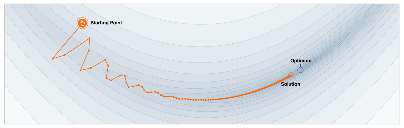
What to do in such situations, and how the GBM regularization parameters are interconnected, as well as the hyperparameters of the basic algorithms, we will describe in the next article. In it, we will analyze the modern packages - xgboost , lightgbm and h2o , and also practice in their proper configuration. In the meantime, we invite you to play around with the GBM settings in another very cool interactive demo: Brliiantly wrong :

5. Homework
Actual homework is announced during the regular session of the course, you can follow in the VC group and in the repository of the course.
As an exercise, complete this task — you need to beat the simple baseline in the Kaggle Inclass competition for predicting departure delays.
6. Useful links
- Open Machine Learning Course. Topic 10. Gradient Boosting
- Video recording of the lecture based on this article.
- Original GBM article from Jerome Friedman
- Chapter in Elements of Statistical Learning by Hastie, Tibshirani, Friedman (p. 337)
- Wiki article about Gradient Boosting
- Frontiers tutorial article about GBM (light-weight PR)
- Hastie Video Lecture about GBM at h2o.ai conference
- Video-lecture by Vladimir Gulin about the composition of algorithms from the Technosphere
- Video lectures by Konstantin Vorontsov ( part 1 , part 2 ) about the composition of algorithms from the School of Data Analysis
Special thanks to yorko (Yuri Kashnitsky) for valuable comments, as well as bauchgefuehl (Anastasia Manokhina) for their help with editing.
')
Source: https://habr.com/ru/post/327250/
All Articles