Scilab in free fall
Recently, I was surprised to find that there are almost no articles on Habré on Scilab. Meanwhile, it is quite a powerful computer math system, open and cross-platform, covering a wide range of engineering and scientific problems. In a number of universities (for example, UrFU, ITMO) it is used to train students. One of the most pressing engineering problems is the solution of differential equations (hereinafter - DE). In this article, I will show how using Scilab to solve systems of ordinary DE using the example of Felix Baumgartner’s famous stratospheric jump simulation.
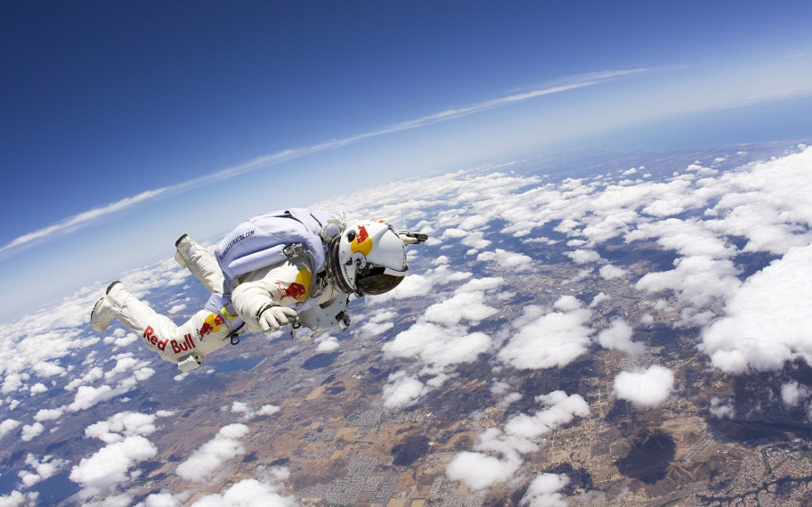
As it is known, free fall is an equally variable movement under the action of gravity, when other forces acting on the body are absent or negligible. In everyday life, movement in the Earth’s atmosphere is also often called free fall, when no force affects the acceleration of the body, except for the air resistance force and the force of gravity. It is this expanded understanding that we will use in the future.
Task
Create differential equations (DM), describing the essential properties of the flight of Baumgartner, solve them with Scilab means and obtain explicitly the dependence of distance and speed on the time of free fall.
Initial data
Since The main task of the article is to show how Scilab can solve an ODE, and not especially get involved in analyzing experimental data (telemetry), errors and fitting. However, to verify the adequacy of the model, several values must still be taken. So:
- The height of the jump - 39000m.
- The distance of free fall is 36402.6m.
- Free fall time - 4 min. 20 sec.
- During the first 20 seconds, Baumgartner picked up a speed of 194 m / s, after 50 seconds of falling (at an altitude of 8447 m), he reached a record speed of 377 m / s, and by the time the parachute opened (ie, after 260 seconds of flight), the speed of fall decreased to 77 m / seconds
Sources: Wikipedia , Press , Video .
Model-1 (excluding air resistance)
Let's start with the simplest model, in which there is only one force - the force of gravity of the Earth. We assume that the fall is strictly vertically, the origin of coordinates is located at the point of the start of the jump, the axis-y is directed downwards.
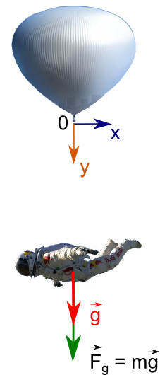
The acceleration of the extremal, respectively, is equal to the acceleration of free fall.
[ ]At the same time, by definition, the speed:
[ ]
Got a system of two ordinary remote control. We decide.
We will use the ode () function included in the standard Scilab distribution.
According to the documentation, ode solves explicit ordinary differential equations defined as:
[ ]
Just like in our case. On the left must be derivatives of the 1st order.
If the remote control contains the derivative of the second, third, and other orders, then you need to introduce replacement (s) and convert one equation with a system of several. As we actually did. After all, acceleration is the 2nd derivative of the time coordinates, from which we moved to the 1st derivative, by introducing a substitution - the variable “speed” equal to dy / dt. Those.
from [ ] switched to $ inline $ \ begin {equation *} \ begin {cases} \ frac {dv} {dt} = g \\ \ frac {dy} {dt} = v \ end {cases} \ end {equation *} $ inline $
Finally go to the code (link to github ). You can write it in the SciNotes editor proposed by the environment, as well as in any other text editor. You can also run a shell without graphics and enter commands in the console. In my opinion, SciNotes is more convenient by highlighting the code and integrating it into the development environment.
First of all, we need to describe the remote control as a function in the Scilab language.
//, //vector = [v,y], t - function dVector = verticalFallingVacuum(t, vector) dVector = zeros(2,1); // - dVector(1) = g; //dv/dt = g dVector(2) = vector(1); //dy/dt = v endfunction Then we set the initial conditions.
// y0 = [0;0]; //v x , / . t0 = 0; // t = 0:0.1:260; // , . (4 20) Then we call the function-solver ode () , passing to it everything that was created above.
result = ode(y0,t0,t,verticalFallingVacuum); // In the result matrix, the result will be the values of the desired function-solutions of this system of remote control, corresponding to points on the time axis from the range specified in t.
Let's look at what happened in graphical form, and at the same time we will display a couple of control points to the console.
// plot(t,result(2,:)); // , xtitle(" "); // // mprintf("C 50 = %f / \n",result(1,500)*3.6); mprintf(" 4.20 = %f \n",result(2,2600)/1000); Together:
g = 9.81; // / mode(0); // //, //vector = [v,y] function dVector=verticalFallingVacuum(t, vector) dVector = zeros(2,1); // dVector(1) = g; //dv/dt = g dVector(2) = vector(1); //dy/dt = v endfunction // y0 = [0;0]; //v x , / . t0 = 0; // t = 0:0.1:260; // , . (4 20) result = ode(y0,t0,t,verticalFallingVacuum); // // plot(t,result(2,:)); xtitle(" ") // mprintf("C 50 = %f / \n",result(1,500)*3.6); mprintf(" 4.20 = %f \n",result(2,2600)/1000); 
The result was the expected quadratic dependence of the coordinate on time.
Check with practice:
Speed in 50 seconds = 1762 km / h (and should be 1357 km / h).
The distance covered is 4min.20sec = 331.3 km (and should be 36.4 km.).
If with a speed at the initial stage of the jump, wrinkling, you can still accept, then the total distance traveled is exceeded by an order of magnitude. This is explained by the fact that the air resistance that we did not take into account in the initial part of the flight is really small due to the stratospheric sparseness and our simplest model somehow cope with it, but as the atmosphere decreases, the density of the atmosphere increases noticeably, the fall rate decreases significantly and the practice begins to completely diverge from theory.
If we construct a more detailed graph, on which we also plot experimental points, then the discrepancy of this model and reality that will worsen with time will become even clearer. In particular, the speed increases linearly, whereas in practice it should start to decrease from a certain point.
Plotter function:
// . //t - 1xN //data - - 2xN v,y //realJumpVT - 2N - -. //realJumpYT - 2xN -. function [yAxis,vAxis] = drawGraphics (t, data, realJumpVT, realJumpYT) scf();// xsetech([0 0 0.9 0.47]);// - - plot2d(t', data(2,:)'); yAxis=gca(); // yAxis.title.text = " , "; yAxis.title.font_size=2; // yAxis.x_label.text = " , "; yAxis.y_label.text = " , "; yAxis.grid = [0,0]; // yAxis.x_location = "origin"; // x- yAxis.y_location = "origin"; // y- yAxis.children(1).children(1).foreground = 11; // plot2d(realJumpYT(2,:), realJumpYT(1,:)',[-2]); // grExpY=gca(); // grExpY.children(1).children(1).mark_foreground = 14; // - grExpY.children(1).children(1).thickness = 2; leg1 = legend(["", " "],-1); xsetech([0 0.53 0.9 0.43]);// - - plot2d(t', data(1,:)'); vAxis=gca(); // vAxis.title.text = " , /"; vAxis.title.font_size=2; // vAxis.x_label.text = " , "; vAxis.y_label.text = " , /"; vAxis.grid = [0,0]; // vAxis.x_location = "origin"; // x- vAxis.y_location = "origin"; // y- vAxis.children(1).children(1).foreground = 11; // - plot2d(realJumpVT(2,:), realJumpVT(1,:)',[-2]); // grExpV=gca(); // grExpV.children(1).children(1).mark_foreground = 14; // - grExpV.children(1).children(1).thickness = 2; plot2d(t', 300*ones(size(t,'c'),1),[3]); // grBarrier=gca(); // grBarrier.children(1).children(1).foreground = 5; // - xstring(200,320," "); t=get("hdl") // //t.font_color=21; // t.font_size=2; leg2 = legend(["", " "],-1); endfunction 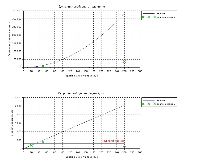
We will correct the situation by introducing the force of air resistance into the model.
Model-2 (including air resistance)
The atmosphere will act on flying with force
[ ]
Where
- resistance coefficient
S - the largest cross-sectional area perpendicular to the direction of flight
density - air density
v - movement speed
The formula is taken from here , where you can also read an analytical solution.
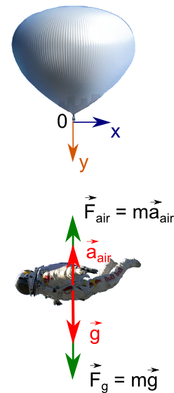
We are interested in acceleration (although it would be better to say slowing down), which F air will report to the flying down extreme in order to add an amendment to the first equation of the system.
According to Newton's 2nd Law [ ]
[ ]
With this amendment, our system will take the form
$$ display $$ \ begin {equation *} \ begin {cases} \ frac {dv} {dt} = g - \ frac {1} {m} \ cdot \ frac {c \ cdot S \ cdot deinsity \ cdot v ^ 2} {2} \\ \ frac {dy} {dt} = v \ end {cases} \ end {equation *} $$ display $$
Solve the same way. We describe the remote control system as a Scilab function.
//, //vector = [v,y], t- function dVector = verticalFallingAir(t, vector) dVector = zeros(2,1); //- height = startHeight-vector(2); // . aAir = (0.5*c*airDensity(height)*S*vector(1)^2)/m; //"" dVector(1) = g - aAtm; //dv/dt = g - aAtm dVector(2) = vector(1); //dy/dt = v endfunction Since the density of the atmosphere varies with altitude, we need to write the appropriate function. The table can be taken from here . In general, there is a GOST 4401-81 Atmosphere standard. Parameters (with a change in N 1).
// function density = airDensity(height) hVSdensity = [ 0 1.225; 50 1.219; 100 1.213; 200 1.202; 300 1.190; 500 1.167; 1000 1.112; 2000 1.007; 3000 0.909; 4000 0.819; 5000 0.736; 8000 0.526; 10000 0.414; 12000 0.312; 15000 0.195; 20000 0.089; 50000 1.027*10^(-3); 100000 5.550*10^(-7); 120000 2.440*10^(-8); ]; // if (height < 0) then height = 0; end // density = interpln(hVSdensity',[height]); endfunction Set the initial conditions and solve.
// step = 0.1; y0 = [0;0]; //v x , / . t0 = 0; // t = 0:step:260; // , . (4 20) result = ode(y0,t0,t,verticalFallingAir); // Build a graph and see what happened.
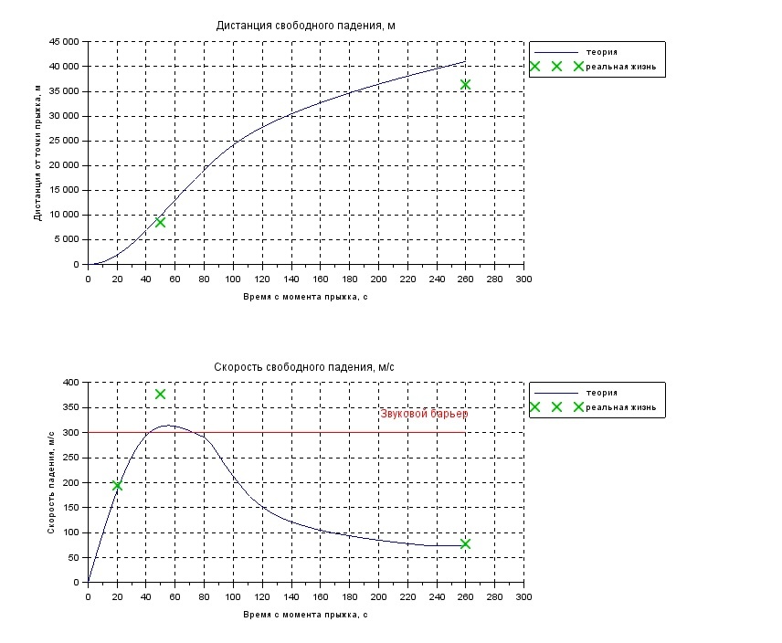
We see that between the 40th and 70th seconds we will break through the sound barrier, in the region of the 50th second the speed will reach a maximum, after which it will begin to decline. Gained speed is not enough to burn in the atmosphere ( discussed at Habré), in addition to the end of the flight speed will drop to a value that allows you to safely open the parachute. What corresponds to reality.
Speed - comparing theory with experiment at control points
| Holy Fall Time, s | Rated speed, m / s | Actual speed, m / s |
|---|---|---|
| 20 | 183 | 194 |
| 50 | 312 | 377 |
| 260 | 73 | 77 |
Holy Fall Distance - Comparison of Theory and Experiment at Control Points
| Holy Fall Time, s | Estimated distance, m | Actual distance, m |
|---|---|---|
| 50 | 9853 | 8447 |
| 260 | 41049 | 36403 |
In terms of speed, the error is on average 27 m / s (7% of the actual record), and in the free fall distance 3026 m (8% of the distance actually traveled in a fall.). For our educational and demonstration purposes is quite acceptable.
Conclusion
Thus, we are an example of a simple, but visual, mat. Models considered how using Scilab to solve remote control, interpolate, build graphs. I hope this article will be useful for beginners to learn Scilab, and some people may be motivated to further use Scilab in their practical activities.
')
Source: https://habr.com/ru/post/327142/
All Articles