Predict the popularity of articles on TJ

Once, on a languid evening, sitting opposite a flashing tjournal tape and sipping chamomile tea, I suddenly found myself reading an article about a Soviet light bulb that had been lighting someone's entrance for 80 years. Yes, very interesting, but I still prefer articles about policy Achievements of AI in the game of doom, the adventures of SpaceX rockets and, in the end, with the highest number of views. And what are all the articles gaining impressive ratings? Posts about the size of a tweet about some kind of political action or talmuda with a detailed analysis of the Russian film industry? Well, then it's time to uncover your Jupyter notebook and display the formula for a perfect article.

Base collection

To get started is to get the data. Since TJ doesn’t have its own API, we’ll collect old good old scraping of bare html using requests and retrieving useful data from it using BeautifulSoup . At the exit we get 39116 articles from 2014. However, it should be noted that the article itself is written in the form of a html block with all its inherent bunch of tags, and not as simple text. The script itself is here .

Feature Engineering

After an hour of the script, we have almost 39,000 articles in our hands, and it is time to pull features from them of all degrees of importance. But first we import everything you need:

import json import datetime import numpy as np import pandas as pd import snowballstemmer from bs4 import BeautifulSoup import itertools from scipy.sparse import csr_matrix, hstack from sklearn.feature_extraction.text import TfidfTransformer, CountVectorizer from sklearn.cross_validation import train_test_split from sklearn.decomposition import LatentDirichletAllocation from gensim.models import Word2Vec import lightgbm as lgb from sklearn.metrics import r2_score, mean_absolute_error import seaborn as sns import matplotlib.pyplot as plt %matplotlib inline 

We read our dataset and see its contents:

 dataframe = pd.read_json("data/tj_dataset.json") dataframe.head() 

Because of the available data for training, we have only the content of the post and the date of publication, then most of the engineering features will revolve around text data. From the post itself you can get two types of features: structural and semantic (yes, the names came up with himself). The structural ones include those that, do not believe, determine the structure of a post: the number of links to YouTube, Twitter, the number of words in the title of the post, the average number of words in text blocks, etc. All values ​​that could not be caught (usually due to the small amount of text data), just replace with -9999, gradient boosting will understand us.

Let's start with temporary features. And here everything is impossible - we pull out the year, month, day, hours and minutes, from engineering the features here only the day of the week:

 def get_time(x): time = x.split()[-1] h, m = time.split(":") return int(h)*60 + int(m) m_keys = { '': 1, '': 2, '': 3, '': 4, '': 5, '': 6, '': 7, '': 8, '': 9, '': 10, '': 11, '': 12, } 

 dataframe['month'] = dataframe.date.apply(lambda x: m_keys[x.split()[1]]) dataframe['time'] = dataframe.date.apply(get_time) dataframe['day'] = dataframe.date.apply(lambda x: int(x.split()[0])) dataframe['year'] = dataframe.date.apply(lambda x: int(x.split()[2][:-1])) dataframe["weekday"] = dataframe[["year", "month", "day"]].apply(lambda x: datetime.date(*x).weekday(), axis=1) 

And now the most creative part of the work has begun, where you can give free rein to your imagination and collect everything from your texts.

First of all, you should remove bare chunks of text from the html block, tokenize them and pass through the resulting words:

 stemmer = snowballstemmer.RussianStemmer() rus_chars = set([chr(i) for i in range(1072, 1104)]) def tokenize_sent(sent): sent = sent.lower() sent = "".join([i if i in rus_chars else " " for i in sent]) words = stemmer.stemWords(sent.split()) return words 

Without thinking twice, we add to the list of features the number of words in the post and title, the number of html tags, the mean and root-mean-square ration of the number of words in the blocks. Posts on tj are full of pictures, videos, references to twitter and links to other resources, which can also be used:

 def get_p_data(article): html = BeautifulSoup(article, "lxml") data = html.findAll("p") return [i.text for i in data] def get_p_count(article): html = BeautifulSoup(article, "lxml") data = html.findAll("p") return len(data) def get_p_sizes(article): html = BeautifulSoup(article, "lxml") data = html.findAll("p") return [len(preprocess_sent(i.text)) for i in data] def get_tags_count(article): html = BeautifulSoup(article, "lxml") data = html.findAll() return len(data) def mean_p(x): if not len(x): return -9999 return np.mean(x) def std_p(x): if not len(x): return -9999 return np.std(x) 

 dataframe['p_list'] = dataframe.article.apply(get_p_data) dataframe['text_chained'] = dataframe.p_list.apply(lambda x: "\n".join(x)) dataframe['p_list_tokenized'] = dataframe.p_list.apply(lambda x: [tokenize_sent(i) for i in x]) dataframe['p_list_tokenized_joined'] = dataframe.p_list_tokenized.apply(lambda x: list(itertools.chain(*x))) dataframe['title_tokenized'] = dataframe.title.apply(tokenize_sent) dataframe['images_count'] = dataframe.article.apply(lambda x: x.count("wrapper-image")) dataframe['wide_labels_count'] = dataframe.article.apply(lambda x: x.count("wrapper-wide")) dataframe['link_widget_count'] = dataframe.article.apply(lambda x: x.count("link-widget")) dataframe['links_count'] = dataframe.article.apply(lambda x: x.count("a href")) - \ (dataframe.images_count + dataframe.link_widget_count) dataframe['youtube_count'] = dataframe.article.apply(lambda x: x.count("wrapper-video")) dataframe['tweets_count'] = dataframe.article.apply(lambda x: x.count("wrapper-tweet")) dataframe["tags_count"] = dataframe.article.apply(get_tags_count) dataframe["p_count"] = dataframe.p_list.apply(len) dataframe["text_sizes"] = dataframe.p_list_tokenized.apply(lambda x: [len(i) for i in x]) dataframe["text_sizes_mean"] = dataframe.text_sizes.apply(mean_p) dataframe["text_sizes_std"] = dataframe.text_sizes.apply(std_p) dataframe["text_words_count"] = dataframe.p_list_tokenized.apply(lambda x: len(list(itertools.chain(*x)))) dataframe["title_words_count"] = dataframe.title_tokenized.apply(lambda x: len(x)) 

Here with semantic features the situation is more complicated. And the first thing that comes to mind: tf-idf - a classic in the processing of text data. But only tf-idf does not inspire confidence, so we will also include Latent Dirihlet Allocation (LDA) to reduce the dimension of the post to a 10-50 element vector. Just in case, we will try to take three LDAs of 10, 20 and 50 topics, respectively.

 count_vec = CountVectorizer(tokenizer = tokenize_sent, min_df=10, max_df=0.95) text_count_vec = count_vec.fit_transform(dataframe.text_chained) text_tfidf_vec = TfidfTransformer().fit_transform(text_count_vec).toarray() lda_features = [] topic_counts = [10, 20, 50] for topics in topic_counts: lda = LatentDirichletAllocation(topics, n_jobs=7, learning_method="batch") feats = lda.fit_transform(text_count_vec) lda_features.append(feats) lda_features = np.concatenate(lda_features, axis=1) 

Can I add something else interesting? Of course, word2vec :

 w2v = Word2Vec(dataframe.p_list_tokenized_joined, size=300, workers=7, min_count=5) w2v_dict = {key:w2v.wv.syn0[val.index] for key, val in w2v.wv.vocab.items()} vectors = list(w2v_dict.values()) words = list(w2v_dict.keys()) words_set = set(words) 

At the exit, we have a bunch of word vectors with 300 elements each. Now you need to somehow use them for the vectorization of the post. To do this, you can use 2 techniques: the calculation of the average vector among all the vectors of words and more complex, using clusters.

From the first, everything is clear - there is a matrix with vectors of words, just take the mean value along the first axis, the algorithm for processing empty posts is about the same as above:

 def get_mean_vec(sent): matrix = [w2v_dict[i] for i in sent if i in words_set] if not matrix: return np.full((300,), -9999) return np.mean(matrix, axis=0) 

From the second, you need to build a certain number of clusters for all the word vectors and then assign each word in the text to belong to a particular cluster, i.e. it will turn out something like CountVectorizer on steroids. Just as in the case of LDA, we will try to take several KMeans with different number of clusters:

 kmeans = [] clusters_counts = [10, 50, 100, 500, 1000] for clusters in clusters_counts: kmeans.append(KMeans(clusters, precompute_distances=True, n_jobs=7).fit(vectors)) 

 word_mappings = [] for kmean in kmeans: labels = kmean.labels_ word_mappings.append(dict(zip(words, labels))) def get_centroids_vec(sent): words = [i for i in sent if i in words_set] if not words: return np.full((sum(clusters_counts),), -9999) result_total = np.asarray([]) for cnt, mapper in zip(clusters_counts, word_mappings): result = np.zeros((cnt, )) for word in words: result[mapper[word]] += 1 result_total = np.concatenate([result_total, result]) return result_total 

 mean_texts = np.asarray([get_mean_vec(s) for s in dataframe.p_list_tokenized_joined.tolist()]) mean_titles = np.asarray([get_mean_vec(s) for s in dataframe.title_tokenized.tolist()]) clusters_texts = np.asarray([get_centroids_vec(s) for s in dataframe.p_list_tokenized_joined.tolist()]) clusters_titles = np.asarray([get_centroids_vec(s) for s in dataframe.title_tokenized.tolist()]) 

All features collected, it remains only to group them together into one large matrix:

 feats = ["time", "day", "weekday", "month", "images_count", "wide_labels_count", "link_widget_count", "links_count", "youtube_count", "tweets_count", "tags_count", "p_count", "text_sizes_mean", "text_sizes_std", "text_words_count", "title_words_count"] X = dataframe[feats].as_matrix() preprocessed_df = np.concatenate([X, mean_texts, mean_titles, lda_features, clusters_texts, clusters_titles], axis=1) full_df = hstack([csr_matrix(preprocessed_df), text_tfidf_vec]).tocsr() 

Model training

Since we have the number of views and rating here, then the regression problem directly arises. Every month the number of subscribers to tj increases, and this means that the number of views is also increasing. Those. you need to somehow normalize the number of views, while minimizing the impact of emissions. To normalize one post, you can take the mean and standard deviation of the previous 200 posts, scale the current value, while removing everything that is behind the first and 99th percentiles:

 hits_y = dataframe.hits step = 200 new_hits = [] for i in range(step, dataframe.shape[0]): hits = hits_y.iloc[i-step: i+1] perc_high = np.percentile(hits, 99) perc_low = np.percentile(hits, 1) hits = hits[(hits > perc_low)&(hits < perc_high)] mean = hits.mean() std = hits.std() val = max(min(hits_y.iloc[i], perc_high), perc_low) new_hits.append((val - mean)/std) hits_y = np.asarray(new_hits) full_df = full_df[step:] 

Look at the distribution of our ratings:

 plt.hist(hits_y, bins=100) 

It is expected bevel to the left. This is usually treated with a logarithm:

 plt.hist(np.log(hits_y - hits_y.min()+1e-8), bins=100) 

Already much better.

 min_val = hits_y.min() hits_log = np.log(hits_y - min_val+1e-6) 

The most difficult thing is over, it remains only to choose a model, put it on training and pray for the right choice of hyper parameters. Usually they don’t bother with choosing a model and immediately take xgboost, which makes sense, because it has already gained its popularity on kaggle and is widely used by both novices and gurus. But one day, accidentally stumbling upon a comparison of benchmarks of two implementations of gradient boosting, Microsoft drew attention to LigthGBM from Microsoft with its delicious test results, which made the old man xgboost be put off as a fallback.

In general, the training is the same as on xgboost - we poke back and forth max_depth and regularization to avoid overfit, we select the best number of trees under the minimum learning_rate.

Dataset for LigthGBM is necessary to start with a local format:

 features = (feats + list(itertools.chain(*[[f"lda_{lda}_{i}" for i in range(lda)] for lda in topic_counts])) + [f"mean_matrix_body_{i}" for i in range(300)] + [f"mean_matrix_title_{i}" for i in range(300)] + list(itertools.chain(*[[f"clusters_body_{i}_{j}" for j in range(i)] for i in clusters_counts])) + list(itertools.chain(*[[f"clusters_title_{i}_{j}" for j in range(i)] for i in clusters_counts])) + [f"tf_idf_{i}" for i in range(text_tfidf_vec.shape[1])]) 

 X_train, X_test, y_train, y_test = train_test_split(full_df, hits_log, test_size=0.2, random_state=753) train_data = lgb.Dataset(X_train, label=y_train, feature_name=features) test_data = train_data.create_valid(X_test, label=y_test) 

Gradient boosting parameters (obtained after long hours of training):

 param = {'num_trees': 100000, 'application':'regression', 'learning_rate': 0.01, 'num_threads': 7, 'max_depth': 10, 'lambda_l2': 1e-3} param['metric'] = 'mae' 

Directly training itself:

 bst = lgb.train(param, train_data, param['num_trees'], valid_sets=[test_data], early_stopping_rounds=200) 

An important feature of trees is that it is possible to appreciate the importance of the features:

 importance = sorted(zip(features, bst.feature_importance()), key=lambda x: x[1], reverse=True) for imp in importance[:20]: print("Feature '{}', importance={}".format(*imp)) 

 Feature 'tags_count', importance=546 Feature 'month', importance=510 Feature 'weekday', importance=431 Feature 'images_count', importance=377 Feature 'lda_20_6', importance=332 Feature 'time', importance=316 Feature 'wide_labels_count', importance=291 Feature 'lda_50_48', importance=227 Feature 'text_sizes_std', importance=215 Feature 'mean_matrix_title_134', importance=174 Feature 'title_words_count', importance=161 Feature 'text_sizes_mean', importance=160 Feature 'lda_20_15', importance=149 Feature 'mean_matrix_body_262', importance=142 Feature 'mean_matrix_body_194', importance=141 Feature 'mean_matrix_title_115', importance=138 Feature 'mean_matrix_body_61', importance=136 Feature 'mean_matrix_title_13', importance=136 Feature 'tf_idf_1427', importance=132 Feature 'lda_10_1', importance=130 

 importance = pd.DataFrame([{"imp": imp, "feat": feat} for feat, imp in importance]) sns.barplot(x="imp", y="feat", data=importance.iloc[:20])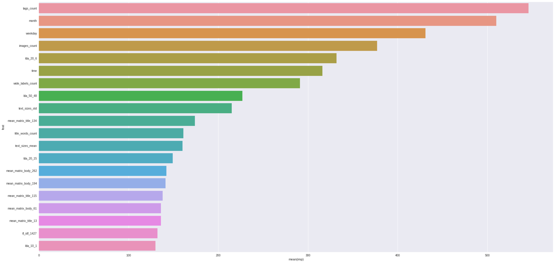 

And here are our results:

 predictions = bst.predict(X_test) print("r2 score = {}".format(r2_score(y_test, predictions))) print("mae error = {}".format(mean_absolute_error(y_test, predictions))) 

 r2 score = 0.3166155559972065 mae error = 0.4209721870443455 

Results

With such parameters and features, the r2 score accuracy is 0.317, and the absolute mean error is 0.42. Is this a good result? Not bad, even considering that there are still ways to improve the model. For example, try neural networks (both recurrent and convolutional, with Embedding layer and word2vec weights), add LDA to PCA, NMF and other decomposition, finally, try to distinguish other features from the category of “ratio of punctuation to number of woo line breaks. " But further research is already leaving you.

UPD.
Here the user ben_yazi indicated in the comments a link to the description of the api for TJ.