Pseudo-toning of images: eleven algorithms and sources

Pseudotoning: Review

About today's theme for programming graphics - pseudo-tinting (dithering, pseudo-mixing colors) - I get a lot of letters, which may seem surprising. You might think that pseudo-toning is not something that programmers should do in 2012. Is pseudo-mixing not an artifact of technology history, an archaism of times, when a display with 16 million colors for programmers and users could only dream about? Why am I writing an article about pseudo-toning in an era when cheap mobile phones work with the brilliance of 32-bit graphics?

In fact, pseudo-toning is still a unique method, not only for practical reasons (for example, preparing a full-color image for printing on a black-and-white printer), but also for an artistic one. Dithering is also used in web design, where this useful method is used to reduce the number of colors in an image, which reduces file size (and traffic) without sacrificing quality. It is also used when reducing digital photos in the RAW format to 48 or 64 bits per pixel to RGB to 24 bits per pixel for editing.

And these are applications only in the field of images. In sound, dithering also plays a key role, but I'm afraid I will not discuss dithering audio here. Only psevdotonirovaniya images.

In this article I am going to focus on three points:
')

• Highlights of image dithering
• Eleven specific two-dimensional dithering formulas, including the well-known level of the Floyd-Steinberg algorithm.
• How to write a general purpose pseudo-mixing engine

Pseudotoning: examples

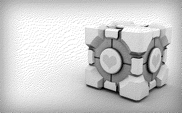
Consider the following full-color image, wallpaper with the famous Companion Cube from the Portal game:


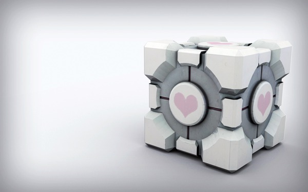
This picture will be the test image for this article. I chose her because she has great combinations of soft gradients and hard edges.

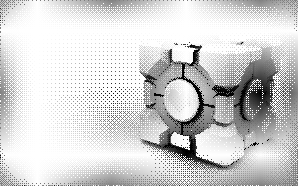
On a modern LCD or LED display - whether it be a computer monitor, smartphone or TV - this full-color image can be output without problems. But let's imagine a PC with more support for a limited color palette. If we try to display our image on such a PC, it might look something like this:


This is the same image as above, but limited to a web palette of safe colors.

Pretty nasty, isn't it? Consider an even more vivid example in which we want to print an image of a cube on a black and white printer. Then we get something like this:


Here the image is barely recognizable.

Problems arise every time an image is displayed on a device that supports fewer colors than the image contains. Subtle gradients in the original image may be replaced by patches of uniform color, and depending on the limitations of the device, the original image may become unrecognizable.

Pseudotoning (or dithering) is an attempt to solve this problem. Psevdotonirovanie works through the approximate expression of inaccessible colors available, for which available colors are mixed so as to simulate inaccessible. As an example, here is an image of a cube, again degraded to the colors of an imaginary old PC, only this time pseudo-toning is applied:


Much better than the non-pseudo-toning version!

If you look closely, you will see that this image uses the same colors as its copy without pseudo-toning. But these few colors are arranged so that it seems as if there are many other colors.

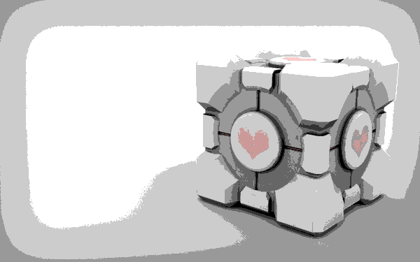
As another example: here is a black and white version of our image with similar pseudo-toning:


Specifically, pseudo-toning using the Sierra two-row algorithm (2-row Sierra) is applied here.

Despite the presence of only black and white colors, we can still discern the shape of the cube down to the hearts on both sides. Dithering is an extremely powerful method and can be used in ANY situation where the data must be presented at a lower resolution than the one for which it was created. This article will focus on images, but the same methods can be applied to any two-dimensional data (or to one-dimensional data, which is even easier!).

The basic concept of pseudo toning

In short, pseudo-toning is fundamentally associated with error dissipation .

Error dispersion works as follows: Suppose we need to reduce the photo in grayscale to black and white colors so that we can print it on a printer that only supports pure black (ink) or pure white (paper without ink) color. The first pixel in the image is dark gray, with a value of 96 on a scale from 0 to 255, where 0 is pure black, 255 is pure white.


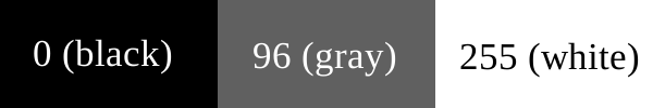
Visualization of RGB values ​​in our example.

When converting such a pixel to black or white, we use a simple formula: is the color value closer to 0 (black) or 255 (white)? 96 is closer to 0 than to 255, so we make the pixel black.

At this stage, the standard approach is to simply move to the next pixel and perform the same comparison. But the problem arises if we have a bunch of similar gray pixels with a value of 96 - they all turn into black. We have a huge piece of empty black pixels that do not represent the original gray color.

Error dispersion follows a smarter approach to the problem. As you might suggest, error dissipation works by “dispersing” - or spreading - the error of each calculation into adjacent pixels. If the algorithm finds a gray pixel with a value of 96, it also determines that 96 is closer to 0 than to 255 - and therefore turns the pixel black. But then the algorithm takes into account the “error” in its conversion. In particular, the error is that the gray pixel that we made black, in fact, was 96 steps away from black.

When it moves to the next pixel, the error dissipation algorithm adds the error of the previous pixel to the current pixel. If the next pixel is also gray 96, instead of turning it black, the algorithm adds error 96 from the previous pixel. This leads to a value of 192, which is actually closer to 255 - and therefore closer to white! Thus, the algorithm makes this pixel white and again takes into account the error. In this case, the error is −63, because 192 is 63 less than 255 — the value by which this pixel was changed.

As the algorithm continues, error dissipation leads to alternation of black and white pixels, which simulates the gray color of the value 96 of this segment quite well. This is much better than coloring all the pixels in a row with black. As a rule, when we finish processing the image string, we discard the error value that we were tracking, and start again with the error “0” from the next image line.

Below is an example of the image of our cube using the described algorithm. In particular, each pixel is converted to black or white, the conversion error is noted and transmitted to the next pixel on the right:


This is the easiest application of pseudo-toning with error dispersion.

Unfortunately, pseudo-toning with error dispersion has its own problems. Be that as it may, psevdotonirovanie always leads to prominent points or to the dotted form. This is an inevitable side effect of working with a small number of available colors — because of their number, these colors will repeat again and again.

In the above simple example of the error dissipation algorithm, another problem is obvious - if you have a block of very similar colors and you push the error just to the right, all the “dots” end up in the same place! This leads to funny dot lines that are almost as distracting as the original pseudo-toning version.

The problem is that we only use one-dimensional error dissipation. Spreading an error only in one direction (to the right), we do not distribute it very well. Since the image has two dimensions (horizontal and vertical), why not direct the error in several directions? This will distribute the error more evenly, which, in turn, will allow to avoid the strange lines of the points considered in the example of the error dispersion above.

Pseudo-tinting with two-dimensional error dissipation

There are many ways to dispel errors in two dimensions. For example, we can spread an error by one or more pixels to the right, left, up, and down.

For ease of calculation, all standard dithering formulas push the error forward only. If you go around pixel by pixel, starting from the upper left corner and moving to the right, there will be no need to take errors back (for example, to the left and / or upward) into account. The reason for this is obvious - if you throw an error back, you have to go back to the pixels that have already been processed, which leads to more errors when moving backwards. The result is an endless cycle of error propagation.

Thus, for the standard cycle behavior (starting from the upper left corner of the image and moving to the right), we want the movement of the pixels to go only to the right and down.


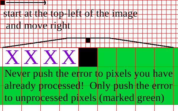
I apologize for the lousy image - but I hope this helps illustrate the essence of correct error propagation.

As for the specific ways of spreading the error, a lot of people were beating smarter than me. Let me share these formulas with you.

(Note: these dither formulas are available on several sites on the Internet, but the most comprehensive reference book I have found is this one .)

Floyd-Steinberg Error Scatter Algorithm

The first and perhaps most well-known error dispersion formula was published by Robert Floyd and Louis Steinberg in 1976. Dispersion of errors occurs as follows:

X 7 3 5 1 (1/16) 

In the above notation, X denotes the current pixel. The fraction at the bottom is the divisor for error. In other words, the Floyd-Steinberg formula can be written as:

  X 7/16 3/16 5/16 1/16 

But such a designation is long and inaccurate, so I will stick to the original.

Let's return to our original example of converting a pixel value from 96 to 0 (black) or to 255 (white). When we color a pixel in black, we get error 96. We spread this error to surrounding pixels, divide 96 by 16 (= 6), then multiply it by the corresponding values, for example:

  X +42 +18 +30 +6 

By spreading the error to several pixels, each with a different value, we minimize all the distracting dotted stripes that are noticeable in the original example of the error dissipation algorithm. Here is an image of a cube using the Floyd-Steinberg algorithm:


Floyd-Steinberg Error Scatter Algorithm

Not bad, huh?

The Floyd-Steinberg error dissipation algorithm is probably the most well known error dissipation algorithm. It gives fairly good quality, and also requires only one front array (a one-dimensional array of image width, where error values ​​are distributed, distributed to the next line). In addition, since its divider is 16, bit shifts can be used instead of division. So the algorithm achieves high speed operation even on old equipment.

As for the 1/3/5/7 values ​​used to propagate the error, they were specially chosen because they create a uniform checkered pattern for the gray image. Clever!

One warning about the Floyd-Steinberg algorithm - some programs may use other, simpler pseudo-toning formulas and call them Floyd-Steinberg, hoping that people do not know the difference. Here's a great dithering article that describes one of these “false Floyd-Steinberg algorithms”:

  X 3 3 2 (1/8) 

This simplification of the original Floyd-Steinberg algorithm gives not only a noticeably worse result, but also does it without any significant advantages in terms of speed (or memory, as an array for storing error values ​​for the next line is still required).

But if you're interested, here is an image of the cube after the passage of the “false Floyd-Steinberg”:


There are far more clusters of points than in the real Floyd-Steinberg algorithm — so don't use this formula!

Algorithm of Jarvis, Judis and Ninke (Jarvis, Judice, Ninke)

In the year when Floyd and Steinberg published their famous dithering algorithm, a less well-known, but much more powerful algorithm was published. The Jarvis, Judith and Ninke filter is much more complicated than the Floyd-Steinberg:

  X 7 5 3 5 7 5 3 1 3 5 3 1 (1/48) 

With this algorithm, the error is distributed to three times more pixels than that of Floyd-Steinberg, which leads to a smoother and more subtle result. Unfortunately, divisor 48 is not a power of two, so bit shifts cannot be applied. Only 1/48, 3/48, 5/48, and 7/48 values ​​are used, so these values ​​can be calculated once and then replicated several times for a small increase in speed.

Another disadvantage of the JJN filter is that it pushes the error down not one line, but two. This means that we need two arrays - one for the next row, the second for the row after it. This was a problem at the time when the algorithm was first published, but on modern PCs and smartphones this additional requirement is irrelevant. Honestly, it may be better to use a single array of image-size errors, rather than erasing two single-row grids over and over again.


Psevdotonirovaniya Jarvis, Judis and Ninke

Dithering Pieces (Stucki)

Five years after the publication of the Jarvis, Judis and Ninke dithering formulas, Peter Stuki published a revised version with minor changes to improve processing time:

  X 8 4 2 4 8 4 2 1 2 4 2 1 (1/42) 

The divisor 42 is not a power of two, but the error dissipation value is yes. Therefore, the error is divided into 42, bit shifts can be used to obtain specific values ​​for dispersion.

For most images, the difference between the Stuck and JJN algorithms will be minimal. Therefore, the former is more often used because of its small speed advantage.


Pseudo-toning Pieces

Dithering atkinson

In the mid-1980s, pseudo-toning became increasingly popular as computer hardware grew to support more powerful video and display drivers. One of the best dithering algorithms of that era was developed by Bill Atkinson, an Apple employee who worked on everything from MacPaint (which he wrote from scratch for the original Macintosh) to HyperCard and QuickDraw.

Atkinson's formula is slightly different from the others on this list, because it spreads only part of the error, not all of it. In modern graphical applications, this method is found under the name "reduce fading." Scattering only part of the error helps to reduce graininess, but continuous light and dark areas of the image can lose color.

  X 1 1 1 1 1 1 (1/8)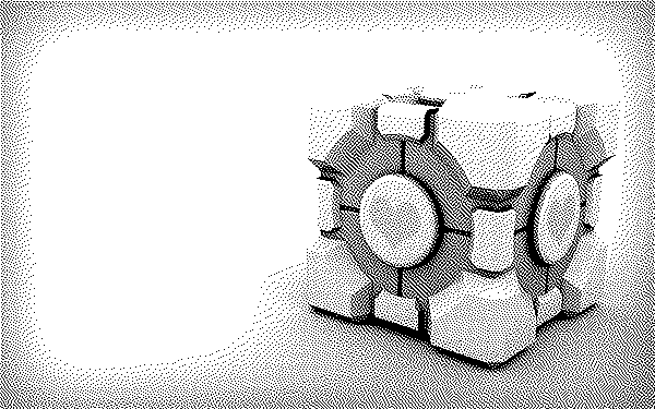 

Psevdotonirovaniya Atkinson

Psevdotonirovaniya Burkes (Burkes)

Seven years after Stucki published improvements to the Jarvis, Judith, and Ninke algorithm, Daniel Burkes suggested further development:

  X 8 4 2 4 8 4 2 (1/32) 

Burkes' proposal was to omit the lower row of the matrix in the Stuck algorithm. This not only eliminated the need for two arrays, but also resulted in a divisor again a multiple of 2. This change meant that all the mathematics involved in the error calculation could be performed by a simple bit shift, and with a slight loss of quality.


Pseudotoning burkes

Psevdotonirovaniya Sierra (Sierra)

The last three dithering algorithms were created by Frank Sierra, who published the following matrices in 1989 and 1990:

  X 5 3 2 4 5 4 2 2 3 2 (1/32) 

  X 4 3 1 2 3 2 1 (1/16) 

  X 2 1 1 (1/4) 

These three filters are commonly referred to as Sierra, Two-Row Sierra (two-row Sierra algorithm) and Sierra Lite. Their final image on the test picture of the cube is as follows:


Sierra (sometimes called Sierra-3)


Two-row Sierra (Sierra's two-row algorithm)


Sierra lite

Other pseudo-toning considerations

If you compare the images above with the pseudo-toning results of another program, you may find small differences. Similar expected. There are surprisingly many variables that can affect the accuracy of the output of the pseudo-toning algorithm. Among them:

• Tracking errors with floating point or integer numbers. Integer methods lose some resolution due to quantization errors.
  
• Reduce bleaching. Some software reduces the error for a given value (perhaps 50% or 75%) to reduce the amount of discoloration of neighboring pixels.
  
• Cut-off threshold for black or white. Values ​​127 or 128 are common, but in some images it may be useful to use other values.
  
• For color images, how brightness is calculated is important. I use the HSL brightness formula ([max (R, G, B) + min (R, G, B)] / 2). Others use ([r + g + b] / 3) or one of the ITU formulas . YUV or CIELAB will achieve even better results.
  
• Gamma correction or other preliminary modifications. It is often useful to normalize an image before converting it to black and white. The choice of method for this will obviously affect the result.
  
• The direction of the cycle. I have discussed the standard approach “from left to right, from top to bottom,” but some smart dithering algorithms will follow a snake-like path, where the direction from left to right is reversed. So you can reduce the spots of homogeneous points and give a more diverse appearance, but they are more difficult to implement.
  

For the sample images in this article, I did not pre-process the original image. All color matches are performed in RGB space with a cutoff of 127 (values ​​<= 127 are set to 0). The cycle direction is standard from left to right from top to bottom.

What specific methods you can use depends on your programming language, processing limitations and the desired result.

I counted 9 algorithms, but you promised 11! Where are the other two?

So far, I have focused exclusively on pseudo-toning on error dissipation, since this method offers better results than static non-diffusion algorithms.

But for the sake of completeness, here are two standard pseudo-toning methods with an ordered blur. Psevdotonirovanie with an orderly blurring leads to a much larger number of points (and worse results) than psevdotonirovanie with the dispersion of errors, but it does not require arrays of the following lines and works very quickly. For more information on pseudo-toning with an ordered blur, see the corresponding article in Wikipedia .


Pseudotoning with ordered blur with 4 × 4 matrix


Psevdotonirovanie with an orderly blur with 8 × 8 matrix

Considering these methods, the article describes 11 different pseudo-toning algorithms.

Writing your own general purpose pseudo-toning algorithm

Earlier this year, I wrote a fully functional pseudo- toning general-purpose generator for PhotoDemon (an open source photo editor). Instead of posting all the code here, let me direct you to the appropriate page on GitHub . The black-and-white image conversion engine starts on line 350. If you have questions about the code that covers the algorithms described on this page, please let me know and I will post additional explanations.

This engine works by allowing you to pre-specify any pseudo-toning matrix in the same way as in this article. Then you pass this matrix to the pseudo-toning engine, and it does the rest.

The engine is designed on the basis of monochrome conversion, but it can be easily modified to work with color palettes. The biggest difference between the color palette situation is that you have to track individual errors for red, green, and blue, and not for one luminance error. Otherwise, all the math is the same.