Let's start with mathematics. Vectorization of calculations in the implementation of technology RAID-6

Many people remember the publication about "Radiks" on Habré "How the developers sat in St. Petersburg and quietly ate mushrooms," in which the partners briefly outlined the history of the appearance of our product. Therefore, in the first article of our Habroblog, we would like to dive into the mathematical foundations of RAIDIX technologies.



Image: www.nonotak.com

Disk array

Many industrial software and hardware systems (enterprise resource management systems, online data analysis, digital content management, etc.) require active data exchange between computers and external data storage devices. The speed of such drives (hard drives) is much lower than the speed of the computer's RAM (and the performance of the entire system, as a rule, rests on its “slowest” component). In this regard, the problem arises of increasing the speed of access to data stored on external devices. Therefore, in practice, the storage subsystem (SHD), combining several independent disks into a single logical device, has become widespread.
')
To improve performance, several disk drives are included in the storage system with the ability to read and write information in parallel. Currently, a family of technologies under the general name RAID is actively used: Redundant Array of Independent / Inexpensive Disks - an excessive array of independent / low-cost hard drives (Chen, Lee, Gibson, Katz, & Patterson, 1993).

These technologies solve not only the task of improving the performance of storage, but also the task accompanying it - improving the reliability of data storage: after all, individual disks can fail when the system is running. Reliability is ensured through information redundancy: the system uses additional disks on which specially calculated checksums are written, allowing information to be restored in the event of a failure of one or more storage disks.

The introduction of redundant disks allows you to solve the problem of reliability, but entails the need to perform additional steps associated with the calculation of checksums with each reading / writing data from disks. The performance of these calculations, in turn, has a significant impact on the performance of the storage system as a whole. In order to increase the performance of RAID computing, the most popular technology in practice is RAID-6, which allows you to recover two failed disks .

This material provides an overview of the RAID technology family and discusses details of the implementation of RAID-6 algorithms on the Intel 64 platform. This information is available in open sources (Anvin, 2009), (Intel, 2012), but we present it in a concise, readable form. In addition, we present the results of comparing the error-tolerant coding library of RAIDIX storage systems with popular libraries that implement similar functionality: ISA-l (Intel), Jerasure (J. Plank).

RAID levels

Computational algorithms that are used in the construction of RAID-arrays, appeared gradually and were first classified in 1993 in the work of Chen, Lee, Gibson, Katz, & Patterson, 1993.

In accordance with this classification, a RAID-0 array is referred to as an independent disk array, in which no measures are taken to protect information from loss. The advantage of such arrays compared to a single disk is the possibility of a significant increase in capacity and performance due to the organization of parallel data exchange.

RAID-1 technology means duplication of each disk of the system. Thus, a RAID-1 array has twice the number of disks as compared to RAID-0, but the failure of one system disk does not entail data loss, since there is a copy for each disk in the array.

RAID-2 and RAID-3 technologies are not widely used in practice, and we will omit their description.

RAID-4 technology involves the use of one additional disk on which the sum (XOR) of the remaining data storage disks is written:

$$

$$P = \ sum_ {i = 0} ^ {N-1} D_i \ begin {aligned} \ qquad where \: N \: - \: number \: disks \: with \: data, \\\: D_i \ : - \: contents of \: i \! - \! Th \: disk \ end {aligned} \ qquad (1)$$

The checksum (or syndrome ) is updated each time data is written to the storage disks . Note that for this there is no need to calculate (1) again, but it is enough to add to the syndrome the difference between the old and the new value of the variable disk. In case of failure of one of the disks, equation (1) can be solved with respect to the appeared unknown, i.e. data from the lost disk will be restored.

Obviously, the read and write operations of the syndrome occur more often than operations with any other data disk. This disk becomes the most loaded element of the array, i.e. weak link in terms of performance. In addition, it wears out faster. To solve this problem, RAID-5 technology was proposed, in which parts of various system disks are used to store syndromes (Fig. 1). Thus, disk loading with read and write operations is leveled.



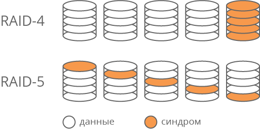
Fig. 1. Difference between RAID-4 and RAID-5

Note that RAID-1 technology — RAID-5 allows you to recover data in the event of a failure of one of the disks, but in the case of the loss of two disks, these technologies are powerless. Of course, the probability of a simultaneous failure of two disks is significantly lower than one. However, in practice, replacing a failed disk requires a certain amount of time during which the data remains “defenseless.” This interval can be very long in the event that system administrators are working in one shift or the system is located in an inaccessible place.

On the other hand, in case of mechanical replacement of the disk, the possibility of human error (replacement of a serviceable disk instead of a failed one), as a result of which we again have the problem of recovering two disks, cannot be excluded. To solve these problems was proposed technology RAID-6, focused on the restoration of two disks. Consider this algorithm in more detail.

RAID-6 technology

The algorithms of calculations used in building storage according to the RAID-6 specification are given in (Anvin, 2009). Here we present them in a form suitable for use within the framework of this study.

In order to increase system performance, data arriving for writing is usually accumulated in the internal storage system cache and written to disks in accordance with the internal caching strategy, which significantly affects the performance of the system as a whole. In this case, write operations are performed by large blocks of data, which will be called stripe in the future.

Similarly to writing, when requesting a physical read from a disk, not only the requested data is read, but also the entire stripe (or several stripes) in which this data is located. In the future, the stripe remains in the system cache, pending read requests related to it.

To improve the performance of the storage stripe is written and read in parallel on all disks of the system. To do this, it is divided into blocks of the same size, which will be denoted $$$D_0, D_1, ..., D_ {N-1}$ . The number of blocks N is equal to the number of data disks in the array. To ensure fault tolerance, two additional disks are introduced into the disk array, which will be denoted P and Q. In the stripe we include the blocks corresponding to the arrays $$$D_0, D_1, ..., D_ {N-1}$ , as well as P and Q disks (Fig. 2.) In case of failure of one or two storage disks, the data in the corresponding blocks are restored using syndromes.



Fig. 2. Stripe structure

Note that in RAID-6 to maintain uniform disk load, as well as in RAID-5 technology, syndromes of different stripes are placed on different physical disks. However, for our research this fact is not relevant. Further, by default, we assume that all syndromes are stored in the last blocks of the stripe.

To calculate the syndromes, we divide the blocks into separate words and repeat the calculation of checksums for all words with the same numbers . For each word, we will calculate the syndromes according to the following rule:

$$

$$\ left \ {\ begin {aligned} P & = \ sum_ {i = 0} ^ {N-1} D_i \\ Q & = \ sum_ {i = 0} ^ {N-1} q_iD_i \ end {aligned } \ right. \ begin {aligned} \ qquad where \: N \: - \: number \: disks \: in \: system, \\ D_i \: - \: block \: data, \: corresponding \: i-volume \: drive, \\ P, Q \: - \: syndromes, \: q_i \: - \: some \: coefficients \ end {aligned} \ qquad (2)$$

Then in the case of the loss of disks with the numbers α and β, you can make the following system of equations:

$$$$ display $$ \ left \ {\ begin {aligned} D_α + D_β & = P - \ sum {} D_i \\ q_αD_α + q_βD_β & = Q - \ sum {} q_iD_i \ end {aligned} \ right. i ≠ α, β; α ≠ β $$ display $$

If the system is uniquely solvable for any α and β, then in the stripe you can restore any two lost blocks. We introduce the following notation:

$$$$ display $$ P_ {α, β} = \ sum_ {i = 0 \\ i ≠ α \\ α ≠ β} ^ {N-1} D_i; \ bar {P} _ {α, β} = P - P_ {α, β} $$ display $$

$$$$ display $$ Q_ {α, β} = \ sum_ {i = 0 \\ i ≠ α \\ α ≠ β} ^ {N-1} q_iD_i; \ bar {Q} _ {α, β} = Q - Q_ {α, β} $$ display $$

Then we have:

$$$$ display $$ \ left \ {\ begin {aligned} D_α + D_β & = \ bar {P} _ {α, β} \\ q_αD_α + q_βD_β & = \ bar {Q} _ {α, β} \ end {aligned} \ right. \ Leftrightarrow \ left \ {\ begin {aligned} D_α & = \ bar {P} _ {α, β} - D_β \\ D_β & = \ frac {q_α \ bar {P} _ {α, β} - \ bar {Q} _ {α, β}} {q_α - q_β} \ end {aligned}, α ≠ β \ right. \ qquad (3) $$ display $$

For the unique solvability (3) it is necessary to ensure that all $$$q_α$ and $$$q_β$ were different and their difference was reversible in the algebraic structure in which the calculations are made. If as such a structure choose the final field $$$GF (2 ^ n)$ (Galois field), then both these conditions coincide with the correct choice of the primitive field element.

If one of the two failed disks contained data and the other a syndrome, then both disks can be recovered using the surviving syndrome. We will not consider this case in detail - the mathematical bases here are similar.

Since in practice the number of disks in the array is not very large (rarely exceeds 100), we can calculate various necessary constants in advance to improve performance.$$ $ inline $ (q_α-q_β) ^ {- 1}, q_α, $ inline $ , and use them further in the calculations.

The speed of performing the calculations in the task in question is crucial for maintaining the overall performance of the storage system not only in the event of a failure of two disks, but also in the “normal” mode, when all disks are operational. This is due to the fact that the stripe is broken into blocks that are physically located on different disks. To read the entire stripe, the operation of parallel reading of blocks from all disks of the system is initiated. When all blocks are read, a stripe is assembled from them, and the stripe reading operation is considered completed. At the same time, the stripe reading time is determined by the last block reading time.

Thus, the degradation of the performance of a single disk entails a degradation of the performance of the entire system. In addition, the slowing down of reading from one disk can be caused by such factors as an unsuccessful head location, an accidentally increased load on the disk, electronically corrected internal disk errors, and many others. To solve this problem, it is possible not to wait until the read operation from the slowest disks of the system is completed, but to calculate their value using the formula (3). However, such calculations will be useful in this situation only if they can be performed fairly quickly.

Note that in the above reasoning it is important for us that the number of the failed disk is obviously known. From a practical point of view, this means that the fact of failure of any disk is detected by hardware control systems, and we do not need to set its number. The task of detecting "hidden" data loss, i.e. data distortions on disks that the system considers to be workable, we have not considered in this material.

It is worth noting that in the term “multiplication” used above, we put a special meaning, different from the multiplication of numbers, to which we are accustomed from school. The classical understanding is not applicable here, because by multiplying two numbers of dimension n bits, as a result we get dimension 2 $$$n$ bit. Therefore, with each subsequent multiplication, the size of the checksum value will increase, and we need the size of all stripe blocks to be the same.

Next, we consider what operations are used in practical calculations, what their complexity is and how they can be optimized.

Arithmetic operations in the final fields

For a detailed assessment of the complexity and reduce the complexity of calculations in the technology of RAID-6, it is necessary to consider in more detail the calculations in the final fields.

We will focus on the fields of the form $$$GF (2 ^ n)$ consisting of $$$2 ^ n$ items. Following (Lidl & Niederreiter, 1988), we present the elements of the field $$$GF (2 ^ n)$ as polynomials with binary coefficients of degree not higher $$$n-1$ . Such polynomials are conveniently written as machine words of bit depth. $$$n$ . We will write them in hexadecimal number system, for example:

$$$$ display $$ x ^ 7 + x ^ 5 + x ^ 2 + 1 → 10100101 → A5 \\ x ^ 5 + x ^ 3 + 1 → 101001 → 29 $$ display $$

It is known that for any n field $$$GF (2 ^ n)$ is obtained by factoring a ring of polynomials over GF (2) modulo an irreducible polynomial of degree $$$n$ . Let's call such a polynomial generator. So the addition in the field $$$GF (2 ^ n)$ can be performed as an operation of addition of polynomials, and multiplication - as an operation of multiplication of polynomials modulo a generating polynomial. Those. the result of multiplying two polynomials is divided by the generating polynomial and the remainder of this division and turns out to be the final result of multiplying two field elements $$$GF (2 ^ n)$ .

An extensive list of irreducible polynomials is given in (Seroussi, 1998). For example, as a generator polynomial for a field $$$GF (2 ^ 8)$ polynomial 171 can be chosen: $$$(x ^ 8 + x ^ 6 + x ^ 5 + x ^ 4 + 1)$ .

Addition operation in $$$GF (2 ^ 8)$ is the same and does not depend on the choice of the generating polynomial, since the degree of the sum cannot exceed the largest of the degrees of the terms. For example:

$$$A5 + 29 = 8C$


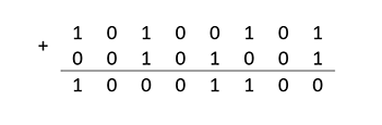
In the case when the degree of the generating polynomial does not exceed the width of the machine word, the operation of adding field elements is performed for one machine instruction of the bitwise exclusive "or".

The multiplication operation is performed in two stages: the elements of the field are multiplied as polynomials, and then the remainder of dividing this product by the generating polynomial is found. For example:

$$$A5 × 29 = 6A (mod 171)$


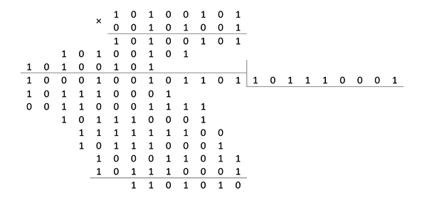
In this case, in terms of elementary machine operations, it is necessary to perform up to 2 (n-1) additions, depending on the value of the factors. It is in this “dependency” that there is a substantial reserve for improving the performance of calculations. For example, if you select
$$$q_i = x ^ {N-i-1}$ , then the calculation of the sum of the form $$$\ sum_ {q_i D_i}$ can be produced according to the Horner scheme:

$$

$$\ sum_ {i = 0} ^ {N-1} x ^ {N-i-1} D_i = (((D_0x + D_1) x + D_2) x + ... + D_ {N-1})$$

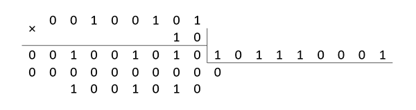
that is, as a multiplier in the multiplication operation, the polynomial can be fixed when calculating syndromes P and Q $$$x$ . Multiplication by polynomial $$$x$ is reduced to a shift operation one digit to the left and adding the result to the module if a shift occurred during the shift. For example:

$$$A5 × 2 = 3B (mod 171)$


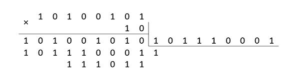
$$$25 × 2 = 4A (mod 171)$


Given the choice $$$q_i = x ^ {N-i-1}$ Formulas (2), (3) can be rewritten as follows:

Calculation of syndromes

$$

$$\ left \ {\ begin {aligned} P & = \ sum {} D_i = D_0 + D_1 + ... + D_ {N-1} \\ Q & = \ sum {} x ^ {Ni-1} D_i = (((D_0x + D_1) x + D_2) x + ... + D_ {N-1}) \ end {aligned} \ right. \ qquad (2 ')$$

Recover two lost data disks

$$$$ display $$ \ left \ {\ begin {aligned} D_α & = \ bar {P} _ {α, β} - D_β \\ D_β & = \ frac {\ bar {P} _ {α, β} - \ bar {Q} _ {α, β} x ^ {α-N + 1}} {1 - x ^ {α-β}} \ end {aligned}, α ≠ β \ right. \ qquad (3 ') $$ display $$

It is important to note that in the calculation of checksums only multiplication operations by $$$x$ and addition. And when restoring data to these operations, several results of multiplication by constants, which are field elements, were also added. The multiplication operation of two arbitrary field elements, which are polynomials of degree less $$$n$ can be rewritten as follows:

$$

$$a (x) b (x) = (a_ {n-1} x ^ {n-1} + a_ {n-2} x ^ {n-2} + ... + a_1x + a_0) (b_ { n-1} x ^ {n-1} + b_ {n-2} x ^ {n-2} + ... + b_1x + b_0) \\ = (((b_ {n-1} a (x) x + b_ {n-1} a (x)) x + b_ {n-3} a (x)) x + ... + b_1a (x)) + b_0a (x)$$

It follows that when restoring data, we only need to be able to add and multiply by $$$x$ . These operations should be carried out with maximum speed.

Vectorization of computations

The fact that we perform the same actions for all data blocks and code words in these blocks allows us to apply various computation vectorization algorithms using Intel processor extensions such as SSE, AVX, AVX2, AVX512. The essence of this approach is that we load several code words into the special vector registers of the processor. For example, if you use SSE with a 128-bit vector register, you can place 16 field elements in one register in one register. $$$GF (2 ^ 8)$ . If the processor supports AVX512, then 64 elements.



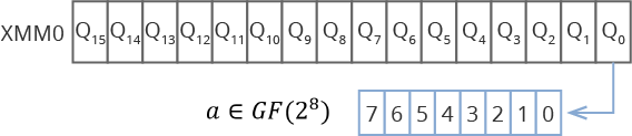
Fig. 3. The location of the data in the vector registers

This idea of ​​locating data in vector registers is used in the calculation in the ISA-L (Intel) and Jerasure (James Plank) libraries. These noise immunity coding libraries are very popular due to their wide functionality and serious optimizations. The multiplication of field elements in these libraries uses the SHUFFLE instruction and auxiliary preexisting “multiplication tables”. A more detailed description of the libraries can be found on Intel and Jerasure sites .

When it comes to vectorization of calculations, the main "art" of the developer is the placement of data in registers. This is where a person still wins compilers.

One of the main advantages of RAIDIX is the original approach, which made it possible to more than double the speed of encoding and decoding data compared to other, already “overclocked” vectorization, libraries. This approach is called “bitwise parallelism” in “Radics”. The company, by the way, has a patent for the appropriate method of calculating and implementing the algorithm.

In RAIDIX, a different approach was applied to vectorization. The essence of the approach is as follows: mentally place vector registers vertically; read from the data blocks of 8 values ​​equal to the size of the register; using SSE, we get 8 * 16 bytes, with AVX - 8 * 32 bytes.



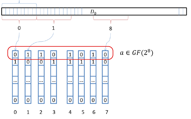
Fig. 4. Vertical allocation of registers

Within the framework of this concept, we have placed in the registers as many field elements as there are bits in one vector register. Multiplication by $$$x$ All elements are immediately executed by three XOR operations and permutation (re-designation) of these 8 registers. In other words, we can multiply 128 or 256 elements of a field by x at once, using just a few simple instructions!



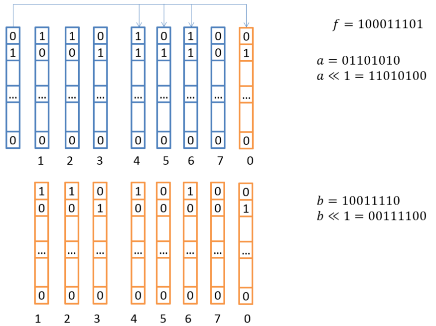
Fig. 5. Scheme of vector multiplication by X

This procedure is repeated for each multiplication by $$$x$ and is used when multiplying by constants. This approach allows encoding and decoding at the highest speed.

We compared RAIDIX algorithms with the most popular ISA-l and Jerasure noise-tolerant coding libraries. The comparison concerned only the speed of the encoding or decoding algorithm - without taking into account the receipt of data from the disks. The comparison was made on a system with the following configuration:

• OC: Debian 8
• CPU: Intel Core i7-2600 3.40GHz
• RAM: 8GB
• Gcc compiler 4.8

In fig. Figure 6 shows a comparison of the encoding and decoding speeds of data in RAID-6 per computing core. The RAIDIX algorithm is referred to as “rdx”. A similar comparison is given for RAID algorithms with three checksums (RAID-7.3).



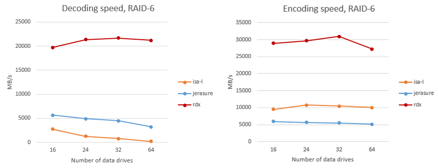
Fig. 6. Comparison of coding and decoding speed in RAID 6



Fig. 7. Comparison of encoding and decoding speed in RAID 7.3

Unlike ISA-L and Jerasure, some parts of which are implemented in Assembler, the RAIDIX library is completely written in C, which allows you to easily transfer the “Radix” code to new or “exotic” types of architecture.

Once again, we note that the numbers reached relate to the same core. The library is perfectly parallelized, and the speed grows almost linearly in multi-core and multi-socket systems.

This implementation of the encoding and decoding operations allows RAID systems to provide reconstruction and write / read performance in the failure mode at the level of several tens of gigabytes per second.

So, as a base data type for vectorization, as a rule, __m128i (SSE) or __m256i (AVX) is used. Since the algorithm uses only simple XOR operations, then, replacing the base type with __m512i (AVX512), the engineers of "Reidix" were able to quickly rebuild, run and test the algorithms on modern multi-core Intel Xeon Phi processors. On the other hand, when using long long (64 bits, standard type C) as the base type, the Radix algorithms are successfully launched on the Russian Elbrus processors.

Literature

1. Anvin, HP (May 21, 2009). The mathematics of RAID-6. Received on November 18, 2009, from The Linux Kernel Archives: ftp.kernel.org/pub/linux/kernel/people/hpa/raid6.pdf
2. Chen, PM, Lee, EK, Gibson, GA, Katz, RH, & Patterson, DA (1993). RAID: High-Performance, Reliable Secondary Storage. Technical Report No. UCB / CSD-93-778. Berkeley: EECS Department, University of California.
3. Intel (1996-1999). Iometer User's Guide, Version 2003.12.16. Obtained 2012, from Iometer project: iometer.svn.sourceforge.net/viewvc/iometer/trunk/IOmeter/Docs/Iometer.pdf?revision=HEAD
4. Intel (2012). The Intel 64 and IA-32 Architects Software Developer's Manual. Vol 1, 2a, 2b, 2c, 3a, 3b, 3c.
5. Seroussi, G. (1998). Table of Low Weight Binary Irreducible Polynomials. Hewlett Packard Computer System Laboratory, HPL-98-135.