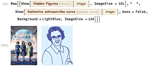
The film "Hidden figures": tasks from the film and a modern approach to the calculations of the orbit and return to Earth

Translated by Jeffrey Bryant, Paco Jain and Michael Trott, " Hidden Figures: Modern Approaches to Orbit and Reentry Calculations ".
The code given in the article can be downloaded here .
I express my deep gratitude to Polina Sologub for assistance in translating and preparing the publication.
Content
- Placement of the satellite in a specific location
- Constants and primary processing
- Calculations
- Plotting
- How are orbits calculated today
Simulation of the returned satellite
The film Hidden Figures, recently released in cinemas, has received good reviews. The action takes place in an important period of US history; It also covers a number of topics such as civil rights and the space race. At the center of the story is the story of Catherine Johnson and her colleagues ( Dorothy Vaughan and Mary Jackson ) from NASA during the deployment of the Mercury program and early research into manned space flight. Attention is also focused on the dramatic struggle for the civil rights of African-American women at NASA, which took place at that time. Computers barely appeared at that time, so the ability of Johnson and her colleagues to solve difficult navigation problems of orbital mechanics without using a computer provided an important test of early computer results.
')
I will focus on two aspects of her scientific work mentioned in the film: orbit calculations and calculations related to entering the atmosphere . For orbital calculations, I first did exactly the same thing as Johnson, and then applied a more modern direct approach using the Wolfram Language tools. The film mentions the solution of differential equations by the Euler method ; I will compare this method with a more modern one and calculate the return trajectory using the data of the atmospheric model, obtained directly from the Wolfram Language).
The film does not cover the details of solving the mathematical problems of the Johnson team, however, what you see is enough to get a feel for and compare the approach displayed in the film with the one that exists at the moment.
Placing a satellite in a specific location
One of the earliest works in which Johnson co-authored (" Determining the azimuth angle at the burnout point to place a satellite over a selected point ") deals with the problem of checking whether a satellite can be placed above a certain point of the Earth after a certain number of orbits around an orbit the starting position (for example, Cape Canaveral, Florida) and the trajectory of rotation. The approach that the Johnson team used to determine the azimuth angle (the angle formed by the velocity vector of the spacecraft at the time of the engine shutdown, with a fixed direction, say, north) to launch the rocket was based on other orbital parameters. This is an important step to ensure the astronaut is properly located to enter the atmosphere on Earth.

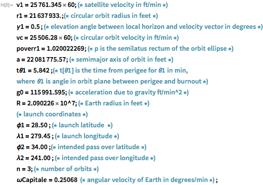
Constants and primary processing
In the article, Johnson defines a series of constants and input parameters necessary for solving the problem manually. Step back a bit to explain the term "burnout", referring to stopping the rocket engine. After the “burnout”, the parameters of the orbit seem to be “frozen”, and the spacecraft moves only under the action of the Earth’s gravity (in accordance with Newton’s laws). In this section, I follow the definitions of units that were adopted in the article.
Some functions for convenience are defined to interact with angles in degrees instead of radians. This allows you to optimize the work when calculating the angles:

Johnson describes several other derived parameters, although it is interesting to note that sometimes she accepts certain values for them, rather than using the values obtained using her formulas. Its values were often close to the values obtained by the formulas. For simplicity, the values from the formulas are used here.
Semilatus rectum elliptical orbit:

The angle in the plane of the orbit between the perigee and the point of burnout:

The eccentricity of the orbit:

Orbit period:

Eccentric anomaly:

To describe the next parameter, it will be easier to quote the original article: "the requirement that a satellite with a burn point φ1, λ1 pass through the selected position φ2, λ2 after completing n orbital passes is equivalent to the requirement that the satellite passes through during the first revolution equivalent place with latitude φ2 as in the selected position, but with λ2 longitude shifted eastwards from λ2 by an amount sufficient to compensate for the Earth’s rotation during n total rotations, i.e. polar hour angle nω E T. The longitude of this equivalent position, therefore, is determined by the ratio ":

Time from perigee for angle θ :

Calculations
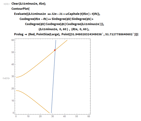
Part of the final decision is to determine the value for the intermediate parameters δλ 1-2 e and θ 2 e . This can be done in several ways. First, I can use ContourPlot to get a graphical solution using equations 19 and 20 of the article:
FindRoot can be used to find numerical solutions:
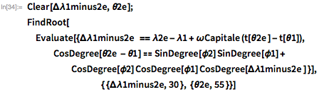

Of course, Johnson did not have access to the ContourPlot or FindRoot functions , so her article describes an iterative method. I translated the methodology described in the article into the Wolfram language, and also revealed a number of other parameters using its iterative method. Since the basic calculations are calculated for the spherical shape of the Earth, the corrections for flattening included:

The graphic representation of the θ 2e value for various iterations demonstrates fast convergence:


I can convert the method in the FindRoot command as follows:


Interestingly, even the iterative steps of finding the root of this more complex system converge fairly quickly:

Plotting
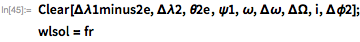
When the orbital parameters are determined, the solution can be visualized. First, from the previous solutions some parameters must be extracted:

Next should be obtained the latitude and longitude of the satellite, depending on the azimuth angle:


φ s and λ s - latitude and longitude as a function of θ s:


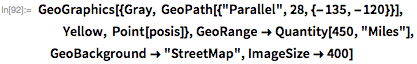
The satellite ground track can be built by creating a table of points:

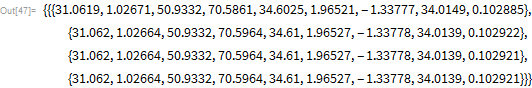
The Johnson article presents an orbital solution scheme, including burnout markers, as well as selected and equivalent positions. This scheme is easy to reproduce:


Here is its original comparison chart:
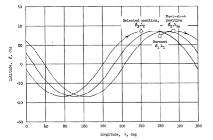
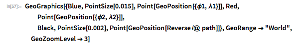
A more visually useful version can be built using the GeoGraphics function, which converts geocentric coordinates to geodesics:


How are orbits calculated today
Today, almost all of us have access to computing resources that are much more powerful than those that NASA had in the 1960s. Now, using only the desktop computer and the Wolfram Language, you can easily find direct numerical solutions of orbital mechanics problems like those that Catherine Johnson and her team were doing.
To calculate the azimuth angle ψ using more modern methods, let's set the parameters for a simple circular orbit originating after burning out over Florida; Let us also assume that the Earth is spherically symmetric (I will not try to search for an exact correspondence with the data from Johnson’s article and redefine some values using the modern system of SI units). Starting from the same height of the near-earth orbit used by Johnson, and using spherical trigonometry, it is easy to derive the initial conditions for our orbit:

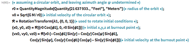
The corresponding physical parameters can be obtained directly using the Wolfram Language:

Then I got the differential equation of motion of our spacecraft, taking into account the gravitational field of the Earth. There are several ways to simulate the gravitational potential near the Earth. Suppose the planet is spherically symmetric and use a Cartesian coordinate system:

In addition, you can use a more realistic model of gravity of the Earth, where the oblate ellipsoid of rotation is taken as the shape of the planet. The exact shape of the potential of such an ellipsoid (assuming a constant mass density of ellipsoidal shells) is available using the EntityValue :

For a common homogeneous triaxial ellipsoid, the potential contains piecewise functions:


Here κ is the largest root of the expression x 2 / (a 2 + κ ) + y 2 / ( b 2 + k ) + z 2 / ( c 2 + κ ) = 1. In the case of a flattened ellipsoid, the previous the formula can be simplified to elementary functions ...

... where κ = ((2 z 2 ( a 2 - c 2 + x 2 + y 2 ) + (- a 2 + c 2 + x 2 + y 2 ) 2 + z 4 ) 1/2 - a 2 - c 2 + x 2 + y 2 + z 2 ) / 2.
The simpler form, which I will use here, is given by the so-called conventional formula for the acceleration of gravity (IGF). This formula takes into account the differences from the spherically symmetric potential up to the second order in spherical harmonics, and gives the results numerically indistinguishable from the exact potential to which they previously referred. In terms of the four measured geodetic parameters, the IGF potential can be determined as follows:
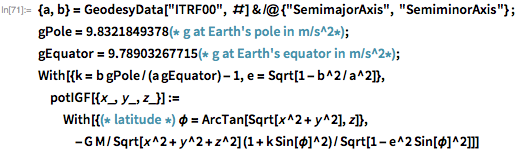
I could easily use even more accurate values for gravity using the GeogravityModelData function. In the initial position, the potential of IGF only by 0.06% deviates from the high order approximation:

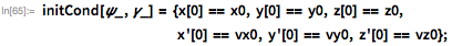
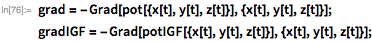
With these functional forms of potential, finding the orbital path requires calculating the potential gradient to obtain a gravitational field vector, then applying Newton's third law. I get the orbital equations of motion for two models of gravity:

Now I am ready to use the power of NDSolve to calculate orbital trajectories. However, before you do this, it will be nice to display the orbital path as a curve in three-dimensional space. To embed these curves in context, I built them on a texture map of the Earth’s surface and projected onto a sphere. Here I built the necessary graphic objects:


While the orbital path, calculated in the inertial reference frame, forms a periodic closed curve, it turns out that the spacecraft will pass through different points on the surface of the Earth during each subsequent revolution. I can visualize this effect by adding extra spin time to the solutions I get from the NDSolve function. Assuming that the number of orbital periods is three (by analogy with the John Glenn flight), I used the Manipulate function to see how the orbital path depends on the azimuth angle, like the study in Johnson’s article. I will build one graph for a spherical Earth (white) and another, green, to demonstrate the effect of oblate (note that the discrepancy increases with each turn):

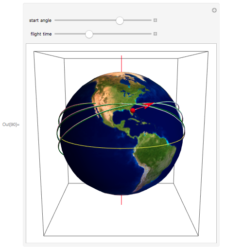
In the document attached to this record, you can see the Manipulate function in action; pay attention to the speed at which each new solution is located. Hopefully, Catherine Johnson and her colleagues at NASA would be impressed!
Now, by changing the angle ψ at the burnout point, it is easy to calculate the position of the spacecraft after, say, three turns:


Simulation of the returned satellite
The film also mentions the Euler method in connection with the return phase. After solving the initial problem of finding the azimuth angle, as was done in the previous sections, it was time to return to Earth. To slow down rotation, rockets are launched, and then, when moving from the airless environment of the cosmos into the atmosphere, a complex set of events occurs. For a cosmonaut to return safely to Earth, factors such as a change in the density of the atmosphere, rapid deceleration and frictional heating should be taken into account. It is necessary to solve the problems of altitude, speed and acceleration as a function of time. This set of problems can be solved using the Euler method, as was done by Catherine Johnson, or using the functionality of solving differential equations in Wolfram Language.
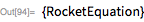
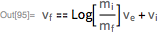
For simple differential equations, a detailed step-by-step solution can be obtained using the specified quadrature method. The equivalent of Newton's well-known formula F = m for the time-dependent mass m (t) is the so-called equation for an ideal rocket (in one dimension) ...
... where m (t) is the mass of the rocket, v e is the exhaust speed of the rocket engine, and m ' p (t) is the derivative of the mass of fuel and time. At constant m ' p (t), the structure of the equation turns out to be relatively simple and easily solvable in closed form:


Having the initial and final conditions for the mass, I get the famous equation of the rocket motion ( K.E. Tsiolkovsky, 1903 ):


Details of the solution of this equation with specific values of the parameters I can take from Wolfram | Alpha . Here are the details along with a comparison with the exact solution, as well as with other methods of numerical integration:


Following the plot of the film, I am now implementing a minimalist model of the re-entry process. We begin by defining parameters that mimic Glenn’s flight:
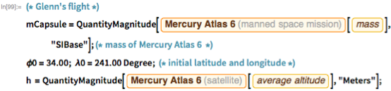
I believe that in the process of braking 1% of the thrust of the engine of the first stage is used, and it lasts, say, 60 seconds. Equation of motion:

Here F grav is the force of gravity, F exhaust ( t ) is the time-dependent force of the engine, and friction force F friction ( x ( t ), v ( t )). The latter depends on both the air density in the x ( t ) position and the friction law for v ( t ).
For air density, which depends on altitude, I can use the StandardAtmosphereData function. I consider it also because of the parachute, which opens at an altitude of about 8.5 km above the ground:

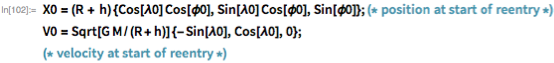
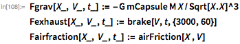
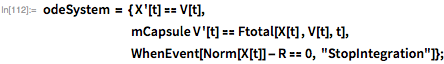
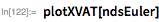
This gives the following set of related non-linear differential equations that need to be solved. The WhenEvent function [...] indicates the end of the construction of a remote control solution when the capsule reaches the surface of the Earth. I use the vector values of the position and velocity of the variables X and V:

Given these definitions for weight, exhaust and air friction, the point of view ...
... the resulting force can be found by:

In this model, I neglected the rotation of the Earth, the internal angles of rotation of the capsule, the active changes in the angle of flight, the supersonic effects of friction force, and many others. The equations solved by Katherine Johnson:


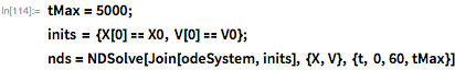
This system of equations is simply solved numerically, if we supplement it with the initial position and velocity. To do this, just refer to the function of NDSolve . I don’t have to worry about the method used, step size control, error control, and so on, because Wolfram Language automatically selects those values that guarantee meaningful results:

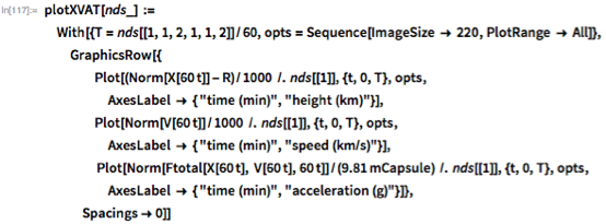
Here is a graph of altitude, speed and acceleration versus time:

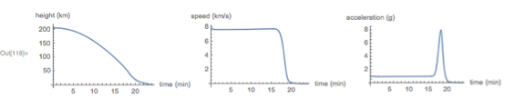
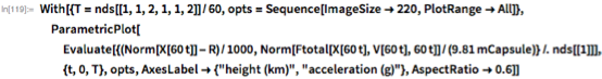
The curve of dependence on height instead of time demonstrates that an exponential increase in air density is responsible for strong inhibition. This is not related to parachuting, which occurs at a relatively low altitude. The deceleration peak occurs at a very high altitude when the capsule quickly transitions from vacuum to atmospheric environment:
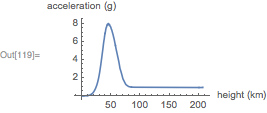
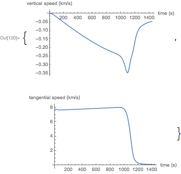
But the graph of the vertical and tangential velocity of the capsule in the process of re-entry:
Now I will repeat the numerical solution by the Euler method with a fixed step:


Qualitatively, this solution looks the same as the previous one:

For the used step size of integration over time, the accumulated error is of the order of several percent. Smaller step sizes will reduce the error:

Note that the landing time predicted by the Euler method deviates by only 0.11% compared to the previous time (for comparison: if I solved the equation with two modern methods, say, BDF or Adams , then the error was would be less by several orders of magnitude).
A large amount of heat is generated during the re-entry process. Here you need a heat shield. At what height is the greatest amount of heat produced per unit area Q ? Without going into details, I can, purely for reasons of dimension, apply the hypothesis
 :
:


A lot of interesting things could be calculated ( Hicks 2009 ), but just as the film was supposed to end, so now I have to complete my article. I hope you forgive me for my words: with the Wolfram Language you can do whatever you want.
Source: https://habr.com/ru/post/326756/
All Articles